Forecasting Temperature with Outliers Imputation

Main goal of the project:

Forecasting temperature in a accurate way using a Machine Learning general approach.

This part of the project will be focused in the following forecasting approaches:

• Forecasting with outliers imputation.

For each approach the best model will be found, applying ML evaluation techniques like cross Validation and hyper-parameter optimization.

Author: Fabio Scielzo Ortiz

Requirements

import polars as pl 
import pandas as pd 
import numpy as np
import sys
import matplotlib.pyplot as plt
import seaborn as sns
sns.set_style("whitegrid")
from statsmodels.tsa.seasonal import STL
import statsmodels.api as sm
from statsmodels.tsa.stattools import adfuller
from statsmodels.graphics.tsaplots import plot_acf, plot_pacf
from datetime import timedelta
from sklearn.metrics import mean_absolute_error
import datetime
import warnings
warnings.filterwarnings("ignore")
import optuna
from PIL import Image
import pickle
import re

from skforecast.ForecasterAutoreg import ForecasterAutoreg 
from skforecast.ForecasterAutoregDirect import ForecasterAutoregDirect
from skforecast.ForecasterAutoregMultiVariate import ForecasterAutoregMultiVariate
from skforecast.ForecasterAutoregMultiSeries import ForecasterAutoregMultiSeries
from sklearn.ensemble import RandomForestRegressor
from sklearn.svm import LinearSVR
from sklearn.linear_model import ElasticNet

sys.path.insert(0, r'C:\Users\fscielzo\Documents\DataScience-GitHub\Time Series')
from PyTS import MakeLags, SARIMA, SimpleExpSmooth, VAR, LinearRegressionTS, KNeighborsRegressorTS, wape, absolute_r2, train_test_split_time_series, OptunaSearchTSCV, time_series_multi_plot, get_prediction_dates, predictive_time_series_plot, KFold_split_time_series, KFold_score_time_series, KFold_time_series_plot, autoSARIMA, DecisionTreeRegressorTS, ExtraTreesRegressorTS, RandomForestRegressorTS, HistGradientBoostingRegressorTS,  MLPRegressorTS, LinearSVRTS, XGBRegressorTS, RidgeTS, LassoTS, ElasticNetTS, StackingRegressorTS, BaggingRegressorTS, OutliersImputer, outliers_time_series_plot

sys.path.insert(0, 'C:/Users/fscielzo/Documents/DataScience-GitHub/EDA')
from EDA import prop_cols_nulls

Data

Conceptual description

Jena Climate is weather time series dataset recorded at the Weather Station of the Max Planck Institute for Biogeochemistry in Jena, Germany.

This dataset is made up of 14 different quantities (such air temperature, atmospheric pressure, humidity, wind direction, and so on) were recorded every 10 minutes, over several years. This dataset covers data from January 1st 2009 to December 31st 2016.

The dataset can be found in Kaggle: https://www.kaggle.com/datasets/mnassrib/jena-climate

Variable Name	Description	Type
Date Time	Date-time reference	Date
p (mbar)	The pascal SI derived unit of pressure used to quantify internal pressure. Meteorological reports typically state atmospheric pressure in millibars.	quantitative
T (degC)	Temperature in Celsius	quantitative
Tpot (K)	Temperature in Kelvin	quantitative
Tdew (degC)	Temperature in Celsius relative to humidity. Dew Point is a measure of the absolute amount of water in the air, the DP is the temperature at which the air cannot hold all the moisture in it and water condenses.	quantitative
rh (%)	Relative Humidity is a measure of how saturated the air is with water vapor, the %RH determines the amount of water contained within collection objects.	quantitative
VPmax (mbar)	Saturation vapor pressure	quantitative
VPact (mbar)	Vapor pressure	quantitative
VPdef (mbar)	Vapor pressure deficit	quantitative
sh (g/kg)	Specific humidity	quantitative
H2OC (mmol/mol)	Water vapor concentration	quantitative
rho (g/m ** 3)	Airtight	quantitative
wv (m/s)	Wind speed	quantitative
max. wv (m/s)	Maximum wind speed	quantitative
wd (deg)	Wind direction in degrees	quantitative

Preprocessing the data

The next piece of code read the data, rename their columns, change the date column to an appropriate date format, ad columns with the day, week, month, quarter and year of each observation and remove the last row which is the only point related with 2017.

climate_df = pl.read_csv(r'C:\Users\fscielzo\Documents\DataScience-GitHub\Time Series\Temperature Prediction\Second Project\Data\jena_climate_2009_2016.csv')

climate_df.columns = ['date', 'p', 'T', 'Tpot', 'Tdew', 'rh', 'VPmax', 'VPact', 'VPdef', 
                      'sh', 'H2OC', 'rho', 'wv', 'max_wv', 'wd']

climate_df = climate_df.with_columns(pl.col("date").str.to_date("%d.%m.%Y %H:%M:%S").name.keep())

climate_df = climate_df.with_columns(climate_df['date'].dt.day().alias('day'),
                        climate_df['date'].dt.month().alias('month'),
                        climate_df['date'].dt.year().alias('year'),
                        climate_df['date'].dt.week().alias('week'),
                        climate_df['date'].dt.quarter().alias('quarter'))

climate_df = climate_df[:-1,:] # removing last row, just because is the only data point regarding 2017

The data has 420550 rows and 20 columns.

climate_df.shape

(420550, 20)

We print a head and tail of the data.

climate_df.head()

shape: (5, 20)

date	p	T	Tpot	Tdew	rh	VPmax	VPact	VPdef	sh	H2OC	rho	wv	max_wv	wd	day	month	year	week	quarter
date	f64	f64	f64	f64	f64	f64	f64	f64	f64	f64	f64	f64	f64	f64	i8	i8	i32	i8	i8
2009-01-01	996.52	-8.02	265.4	-8.9	93.3	3.33	3.11	0.22	1.94	3.12	1307.75	1.03	1.75	152.3	1	1	2009	1	1
2009-01-01	996.57	-8.41	265.01	-9.28	93.4	3.23	3.02	0.21	1.89	3.03	1309.8	0.72	1.5	136.1	1	1	2009	1	1
2009-01-01	996.53	-8.51	264.91	-9.31	93.9	3.21	3.01	0.2	1.88	3.02	1310.24	0.19	0.63	171.6	1	1	2009	1	1
2009-01-01	996.51	-8.31	265.12	-9.07	94.2	3.26	3.07	0.19	1.92	3.08	1309.19	0.34	0.5	198.0	1	1	2009	1	1
2009-01-01	996.51	-8.27	265.15	-9.04	94.1	3.27	3.08	0.19	1.92	3.09	1309.0	0.32	0.63	214.3	1	1	2009	1	1

climate_df.tail()

shape: (5, 20)

date	p	T	Tpot	Tdew	rh	VPmax	VPact	VPdef	sh	H2OC	rho	wv	max_wv	wd	day	month	year	week	quarter
date	f64	f64	f64	f64	f64	f64	f64	f64	f64	f64	f64	f64	f64	f64	i8	i8	i32	i8	i8
2016-12-31	1000.11	-3.93	269.23	-8.09	72.6	4.56	3.31	1.25	2.06	3.31	1292.41	0.56	1.0	202.6	31	12	2016	52	4
2016-12-31	1000.07	-4.05	269.1	-8.13	73.1	4.52	3.3	1.22	2.06	3.3	1292.98	0.67	1.52	240.0	31	12	2016	52	4
2016-12-31	999.93	-3.35	269.81	-8.06	69.71	4.77	3.32	1.44	2.07	3.32	1289.44	1.14	1.92	234.3	31	12	2016	52	4
2016-12-31	999.82	-3.16	270.01	-8.21	67.91	4.84	3.28	1.55	2.05	3.28	1288.39	1.08	2.0	215.2	31	12	2016	52	4
2016-12-31	999.81	-4.23	268.94	-8.53	71.8	4.46	3.2	1.26	1.99	3.2	1293.56	1.49	2.16	225.8	31	12	2016	52	4

We make a fast descriptive summary of the data.

climate_df.describe()

shape: (9, 21)

describe	date	p	T	Tpot	Tdew	rh	VPmax	VPact	VPdef	sh	H2OC	rho	wv	max_wv	wd	day	month	year	week	quarter
str	str	f64	f64	f64	f64	f64	f64	f64	f64	f64	f64	f64	f64	f64	f64	f64	f64	f64	f64	f64
"count"	"420550"	420550.0	420550.0	420550.0	420550.0	420550.0	420550.0	420550.0	420550.0	420550.0	420550.0	420550.0	420550.0	420550.0	420550.0	420550.0	420550.0	420550.0	420550.0	420550.0
"null_count"	"0"	0.0	0.0	0.0	0.0	0.0	0.0	0.0	0.0	0.0	0.0	0.0	0.0	0.0	0.0	0.0	0.0	0.0	0.0	0.0
"mean"	null	989.212751	9.450181	283.492779	4.955886	76.00826	13.576273	9.533771	4.042419	6.022418	9.640238	1216.062557	1.702225	3.056558	174.743714	15.713359	6.51732	2012.496802	26.617729	2.506375
"std"	null	8.358475	8.423346	8.504449	6.730651	16.476195	7.739016	4.184158	4.896855	2.656135	4.235388	39.975064	65.446792	69.017014	86.681794	8.799074	3.448315	2.289752	15.060659	1.116766
"min"	"2009-01-01"	913.6	-23.01	250.6	-25.01	12.95	0.95	0.79	0.0	0.5	0.8	1059.45	-9999.0	-9999.0	0.0	1.0	1.0	2009.0	1.0	1.0
"25%"	null	984.2	3.36	277.43	0.24	65.21	7.78	6.21	0.87	3.92	6.29	1187.49	0.99	1.76	124.9	8.0	4.0	2010.0	14.0	2.0
"50%"	null	989.58	9.42	283.47	5.22	79.3	11.82	8.86	2.19	5.59	8.96	1213.79	1.76	2.96	198.1	16.0	7.0	2012.0	27.0	3.0
"75%"	null	994.72	15.47	289.53	10.07	89.4	17.6	12.35	5.3	7.8	12.49	1242.77	2.86	4.74	234.1	23.0	10.0	2014.0	40.0	4.0
"max"	"2016-12-31"	1015.35	37.28	311.34	23.11	100.0	63.77	28.32	46.01	18.13	28.82	1393.54	28.49	23.5	360.0	31.0	12.0	2016.0	53.0	4.0

There is an anomaly in the variable wv, since the minimum value of it is -9999 when it should be a positive variable since is measure in m/s. We are going to clean this anomaly (error) substituting this value by the mean of the variable.

Naturally, this anomaly has been transmitted to max_wv, so, we will clean this variable as well.

climate_df = climate_df.with_columns(
                        pl.when(pl.col('wv') == pl.col('wv').min())
                        .then(pl.col('wv').mean())  # The replacement value for when the condition is True
                        .otherwise(pl.col('wv'))  # Keeps original value when condition is False
                        .alias('wv')  # Rename the resulting column back to 'variable'
                    )

climate_df = climate_df.with_columns(
                        pl.when(pl.col('max_wv') == pl.col('max_wv').min())
                        .then(pl.col('max_wv').mean())  # The replacement value for when the condition is True
                        .otherwise(pl.col('max_wv'))  # Keeps original value when condition is False
                        .alias('max_wv')  # Rename the resulting column back to 'variable'
                    )

# climate_df.write_csv(r'C:\Users\fscielzo\Documents\DataScience-GitHub\Time Series\Temperature Prediction\Second Project\Data\jena_climate_cleaned.csv')

Checking if the last transformation has solved the anomaly completely.

climate_df.min()

shape: (1, 20)

date	p	T	Tpot	Tdew	rh	VPmax	VPact	VPdef	sh	H2OC	rho	wv	max_wv	wd	day	month	year	week	quarter
date	f64	f64	f64	f64	f64	f64	f64	f64	f64	f64	f64	f64	f64	f64	i8	i8	i32	i8	i8
2009-01-01	913.6	-23.01	250.6	-25.01	12.95	0.95	0.79	0.0	0.5	0.8	1059.45	0.0	0.0	0.0	1	1	2009	1	1

Checking if there are missing values.

prop_cols_nulls(climate_df)

shape: (1, 20)

date	p	T	Tpot	Tdew	rh	VPmax	VPact	VPdef	sh	H2OC	rho	wv	max_wv	wd	day	month	year	week	quarter
f64	f64	f64	f64	f64	f64	f64	f64	f64	f64	f64	f64	f64	f64	f64	f64	f64	f64	f64	f64
0.0	0.0	0.0	0.0	0.0	0.0	0.0	0.0	0.0	0.0	0.0	0.0	0.0	0.0	0.0	0.0	0.0	0.0	0.0	0.0

We can see that there are non missing values in the data, which is specially important.

''''
# If the data would have missing values, a way to fill them could be this:

climate_df = climate_df.fill_null(strategy="forward") # fill NaN's with the previous values 
climate_df = climate_df.fill_null(strategy="backward") # fill NaN's with the later values 
'''

'\'\n# If the data would have missing values, a way to fill them could be this:\n\nclimate_df = climate_df.fill_null(strategy="forward") # fill NaN\'s with the previous values \nclimate_df = climate_df.fill_null(strategy="backward") # fill NaN\'s with the later values \n'

Daily time series

In this section we are going to compute the daily time series for the series with which we are going to work.

df = {}
variables_forecasting = ['T', 'rh', 'VPact', 'H2OC', 'wv', 'max_wv', 'wd', 'p']
for col in variables_forecasting:
    df[col] = climate_df.group_by(['year', 'month', 'day']).agg(pl.col(col).mean()).sort(['year', 'month', 'day'])
    df[col] = df[col].with_columns((pl.col("day").cast(str) + '-' + pl.col("month").cast(str) + '-' + pl.col("year").cast(str)).alias("date"))
    df[col] = df[col].with_columns(pl.col("date").str.to_date("%d-%m-%Y").name.keep())

for col in variables_forecasting:
    print('--------------------------------------')
    print(f'head-tail of {col}')

    display(df[col].head(3))
    display(df[col].tail(3))

--------------------------------------
head-tail of T

shape: (3, 5)

year	month	day	T	date
i32	i8	i8	f64	date
2009	1	1	-6.810629	2009-01-01
2009	1	2	-3.728194	2009-01-02
2009	1	3	-5.271736	2009-01-03

shape: (3, 5)

year	month	day	T	date
i32	i8	i8	f64	date
2016	12	29	2.67625	2016-12-29
2016	12	30	-1.706597	2016-12-30
2016	12	31	-2.4925	2016-12-31

--------------------------------------
head-tail of rh

shape: (3, 5)

year	month	day	rh	date
i32	i8	i8	f64	date
2009	1	1	91.086014	2009-01-01
2009	1	2	92.086806	2009-01-02
2009	1	3	76.458056	2009-01-03

shape: (3, 5)

year	month	day	rh	date
i32	i8	i8	f64	date
2016	12	29	90.384722	2016-12-29
2016	12	30	92.927083	2016-12-30
2016	12	31	74.360694	2016-12-31

--------------------------------------
head-tail of VPact

shape: (3, 5)

year	month	day	VPact	date
i32	i8	i8	f64	date
2009	1	1	3.355524	2009-01-01
2009	1	2	4.267292	2009-01-02
2009	1	3	3.107708	2009-01-03

shape: (3, 5)

year	month	day	VPact	date
i32	i8	i8	f64	date
2016	12	29	6.705833	2016-12-29
2016	12	30	5.048542	2016-12-30
2016	12	31	3.765069	2016-12-31

--------------------------------------
head-tail of H2OC

shape: (3, 5)

year	month	day	H2OC	date
i32	i8	i8	f64	date
2009	1	1	3.357832	2009-01-01
2009	1	2	4.26875	2009-01-02
2009	1	3	3.111944	2009-01-03

shape: (3, 5)

year	month	day	H2OC	date
i32	i8	i8	f64	date
2016	12	29	6.613542	2016-12-29
2016	12	30	4.996875	2016-12-30
2016	12	31	3.749444	2016-12-31

--------------------------------------
head-tail of wv

shape: (3, 5)

year	month	day	wv	date
i32	i8	i8	f64	date
2009	1	1	0.778601	2009-01-01
2009	1	2	1.419514	2009-01-02
2009	1	3	1.250903	2009-01-03

shape: (3, 5)

year	month	day	wv	date
i32	i8	i8	f64	date
2016	12	29	0.837986	2016-12-29
2016	12	30	1.138125	2016-12-30
2016	12	31	0.803403	2016-12-31

--------------------------------------
head-tail of max_wv

shape: (3, 5)

year	month	day	max_wv	date
i32	i8	i8	f64	date
2009	1	1	1.378252	2009-01-01
2009	1	2	2.227361	2009-01-02
2009	1	3	2.065069	2009-01-03

shape: (3, 5)

year	month	day	max_wv	date
i32	i8	i8	f64	date
2016	12	29	1.394028	2016-12-29
2016	12	30	1.839306	2016-12-30
2016	12	31	1.453542	2016-12-31

--------------------------------------
head-tail of wd

shape: (3, 5)

year	month	day	wd	date
i32	i8	i8	f64	date
2009	1	1	181.863077	2009-01-01
2009	1	2	125.072014	2009-01-02
2009	1	3	190.383333	2009-01-03

shape: (3, 5)

year	month	day	wd	date
i32	i8	i8	f64	date
2016	12	29	196.642639	2016-12-29
2016	12	30	201.359028	2016-12-30
2016	12	31	194.592153	2016-12-31

--------------------------------------
head-tail of p

shape: (3, 5)

year	month	day	p	date
i32	i8	i8	f64	date
2009	1	1	999.145594	2009-01-01
2009	1	2	999.600625	2009-01-02
2009	1	3	998.548611	2009-01-03

shape: (3, 5)

year	month	day	p	date
i32	i8	i8	f64	date
2016	12	29	1013.957569	2016-12-29
2016	12	30	1010.460278	2016-12-30
2016	12	31	1004.476181	2016-12-31

Now we build a data frame with each one of the daily time series (just the values, not th dates).

df_multi = pl.concat([pl.DataFrame(df[col][col]) for col in variables_forecasting], how='horizontal')
df_multi

shape: (2_920, 8)

T	rh	VPact	H2OC	wv	max_wv	wd	p
f64	f64	f64	f64	f64	f64	f64	f64
-6.810629	91.086014	3.355524	3.357832	0.778601	1.378252	181.863077	999.145594
-3.728194	92.086806	4.267292	4.26875	1.419514	2.227361	125.072014	999.600625
-5.271736	76.458056	3.107708	3.111944	1.250903	2.065069	190.383333	998.548611
-1.375208	89.417361	4.938958	4.997014	1.720417	3.564861	213.069861	988.510694
-4.867153	86.260417	3.806736	3.847778	3.800278	5.94	118.287361	990.405694
-15.482847	83.774722	1.5425	1.547083	1.226806	2.097708	156.915486	997.052986
-15.734375	85.659722	1.720972	1.731458	0.7225	1.483333	161.920486	993.506389
-9.609167	87.582639	2.601181	2.593542	0.870208	1.443611	182.944444	1002.969653
-12.301458	83.97625	2.019653	2.013819	0.663819	1.237778	166.947917	1003.113333
-10.728264	82.340833	2.239236	2.232847	0.666458	1.306597	161.756181	1002.967569
-8.681667	83.409306	2.653125	2.6425	1.235	2.289861	163.999861	1004.0075
-5.384861	72.444167	2.926528	2.930694	2.459931	3.696806	190.859722	998.494722
…	…	…	…	…	…	…	…
-0.617431	86.866042	5.064375	5.066875	1.433264	2.237917	166.400903	999.409931
-1.665556	83.265694	4.479583	4.473681	1.436042	2.364236	184.094236	1001.110556
-0.007361	86.631944	5.287292	5.271875	2.062569	3.229583	183.505556	1002.849028
1.245069	90.029861	6.014097	5.977778	1.566042	2.468681	180.311667	1005.972569
4.539514	80.470833	6.804236	6.820486	3.030694	5.145972	210.6925	997.729375
7.798611	78.586111	8.357917	8.392361	2.673472	5.390069	222.744306	995.797778
7.527431	75.522778	7.959167	7.977153	3.428889	6.124236	231.709028	998.122569
5.245625	72.531806	6.474306	6.428611	3.067083	6.255069	258.195139	1006.777708
4.887153	84.070833	7.269583	7.171875	2.558194	4.726597	254.427708	1013.542986
2.67625	90.384722	6.705833	6.613542	0.837986	1.394028	196.642639	1013.957569
-1.706597	92.927083	5.048542	4.996875	1.138125	1.839306	201.359028	1010.460278
-2.4925	74.360694	3.765069	3.749444	0.803403	1.453542	194.592153	1004.476181

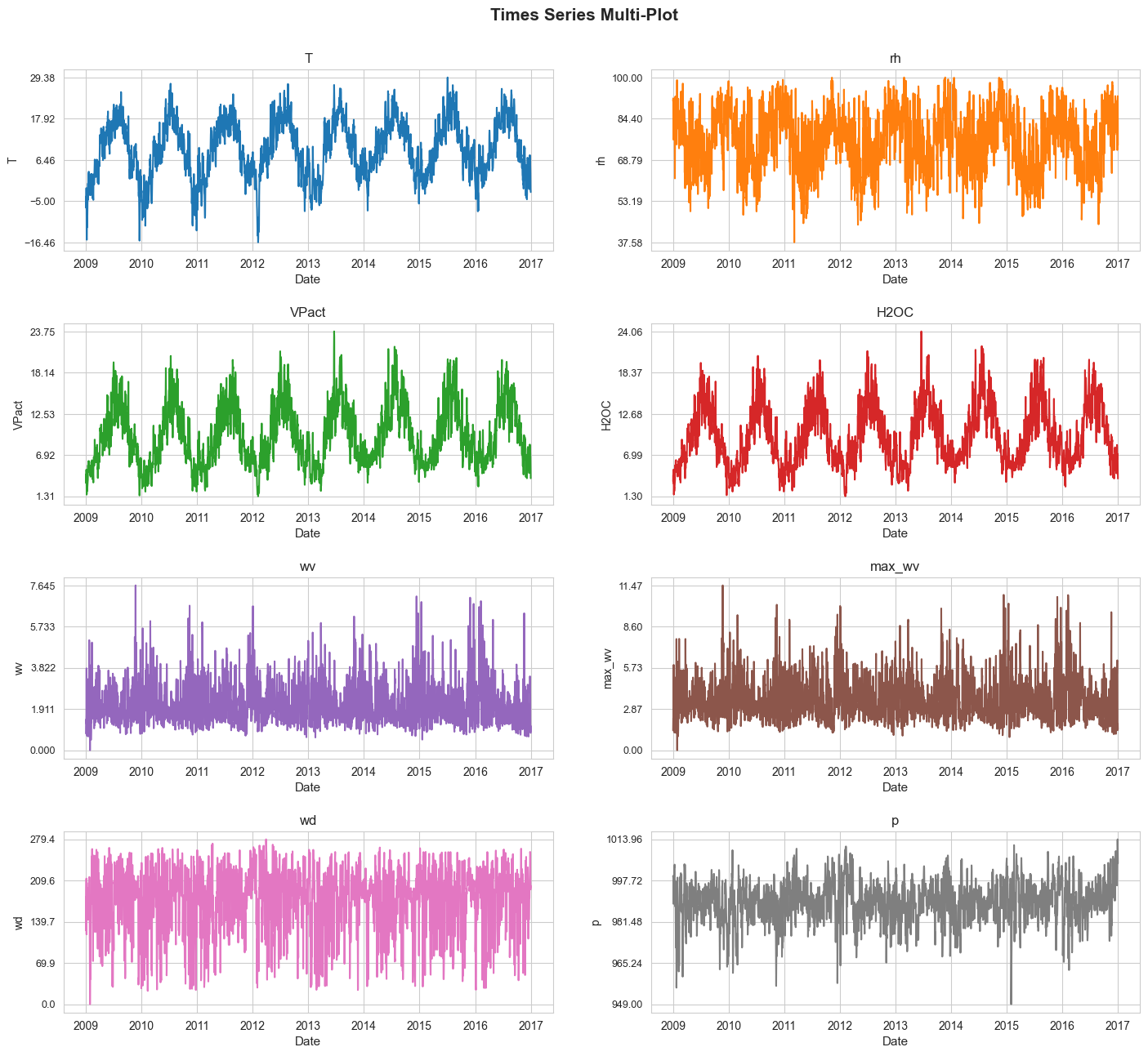
Plotting

In this section we are going to plot all the considered time series as a multi-plot.

time_series_multi_plot(df=df, n_cols=2, figsize=(17, 15), title='Times Series Multi-Plot', 
                       titles_size=15, title_height=0.93, 
                       subtitles_size=12, hspace=0.4, wspace=0.2)

Outlier detection and imputation

PyTS incorporates tools for outliers detection and imputation in Time Series.

The idea of this methods is to detect extreme values in a given series (using the Tukey rule so far), and substitute (impute) them by mean of different strategies.

The current strategies available for imputing the outliers are:

• Trend: the outliers are imputed using the trend of the original series.

• Model: the outliers are imputed using the estimations of a given model for those points.

The main goals of this section are:

• Illustrates how the outlier detection and imputation methods work visually.

• Try outliers imputations as another alternative for forecasting the temperature in Jena 15 days ahead.

  • Basically, we are going to follow the schema of the above sections but applying outliers imputations as a first step in the pipeline.

  • We want to investigate if this preprocessing step could improve the predictive performance of some models.

Visualization

Y, X_st, = {}, {}
X_sk, Y_sk, = {col: {} for col in variables_forecasting}, {col: {} for col in variables_forecasting}
# Defining a grid of lags to be considered as hyper-parameters
lags_grid = [5, 10, 15, 20, 30, 40, 50]

############################################################################
# For univariate forecasting
############################################################################

for col in variables_forecasting:
    # Original series 
    Y[col] = df[col][col].to_numpy()
    # Fake X for statsmodels based implementations
    X_st[col] = np.zeros((len(Y[col]), 4))
                            
    # Lagged X and Y for sklearn based implementations
    for lag in lags_grid:
        make_lags = MakeLags(n_lags=lag, ascending=True)
        make_lags.fit()
        X_sk[col][lag], Y_sk[col][lag] = make_lags.transform(y=Y[col])

outliers_time_series_plot(figsize=(12,9), 
                          outliers_imputer=OutliersImputer(method='trend', period=7, h=1),
                          y=Y['T'], dates=df['T']['date'], 
                          title='Outlier detection and imputation - Daily Avg. Temperature',
                          titles_size=14, subtitles_size=12, hspace=0.4, bbox_to_anchor=(0.5,0.01),
                          legend_size=11)

outliers_time_series_plot(figsize=(12,9), 
                          outliers_imputer=OutliersImputer(method='trend', period=7, h=1),
                          y=Y['T'], dates=df['T']['date'], 
                          title='Outlier detection and imputation - Daily Avg. Temperature',
                          titles_size=14, subtitles_size=12, hspace=0.4, bbox_to_anchor=(0.5,0),
                          zoom_start_date='2008-12-15', zoom_end_date='2011-3-30', title_height=0.97)

outliers_time_series_plot(figsize=(12,9), 
                          outliers_imputer=OutliersImputer(method='model', estimator=SimpleExpSmooth(smoothing_level=0.05), h=1),
                          y=Y['T'], dates=df['T']['date'], X=X_st['T'],
                          title='Outlier detection and imputation - Daily Avg. Temperature',
                          titles_size=14, subtitles_size=12, hspace=0.4, bbox_to_anchor=(0.5,0.01),
                          legend_size=11)

outliers_time_series_plot(figsize=(12,9), 
                          outliers_imputer=OutliersImputer(method='model', estimator=SimpleExpSmooth(smoothing_level=0.01), h=1),
                          y=Y['T'], dates=df['T']['date'], X=X_st['T'],
                          title='Outlier detection and imputation - Daily Avg. Temperature',
                          titles_size=14, subtitles_size=12, hspace=0.4, bbox_to_anchor=(0.5,0.01),
                          legend_size=11)

outliers_time_series_plot(figsize=(12,9), 
                          outliers_imputer=OutliersImputer(method='model', 
                                                           estimator=SARIMA(p=0, d=0, q=1, P=0, D=0, Q=0, s=0), h=1),
                          y=Y['T'], dates=df['T']['date'], X=X_st['T'],
                          title='Outlier detection and imputation - Daily Avg. Temperature',
                          titles_size=14, subtitles_size=12, hspace=0.4, bbox_to_anchor=(0.5,0.01),
                          legend_size=11)

outliers_time_series_plot(figsize=(12,9), 
                          outliers_imputer=OutliersImputer(method='model', 
                                                           estimator=SARIMA(p=0, d=0, q=1, P=0, D=0, Q=0, s=0), h=1),
                          y=Y['T'], dates=df['T']['date'], X=X_st['T'],
                          title='Outlier detection and imputation - Daily Avg. Temperature',
                          titles_size=14, subtitles_size=12, hspace=0.4, bbox_to_anchor=(0.5,0.01),
                          zoom_start_date='2009-11-01', zoom_end_date='2011-04-01', title_height=0.97, legend_size=11)

outliers_time_series_plot(figsize=(12,9), 
                          outliers_imputer=OutliersImputer(method='model', 
                                                           estimator=SARIMA(p=0, d=0, q=1, P=0, D=1, Q=1, s=14), h=0.70),
                          y=Y['T'], dates=df['T']['date'], X=X_st['T'],
                          title='Outlier detection and imputation - Daily Avg. Temperature',
                          titles_size=14, subtitles_size=12, hspace=0.4, bbox_to_anchor=(0.5,0.01),
                          legend_size=11)

Inner evaluation

outer_test_window = 15
inner_test_window = 15
n_splits = 10

Defining the data

# For Sklearn implementations
X_train_sk, X_test_sk, Y_train_sk, Y_test_sk = {col: {} for col in variables_forecasting}, {col: {} for col in variables_forecasting}, {col: {} for col in variables_forecasting}, {col: {} for col in variables_forecasting}

# Train-Test split for univariate forecasting with Sklearn based implementations
for col in variables_forecasting:
    for lag in lags_grid:

        X_train_sk[col][lag], X_test_sk[col][lag], Y_train_sk[col][lag], Y_test_sk[col][lag] = train_test_split_time_series(X=X_sk[col][lag], 
                                                                                                                            y=Y_sk[col][lag], 
                                                                                                                            test_window=outer_test_window)

# For Statmodels implementations
X_train_st, X_test_st, Y_train_st, Y_test_st, = {}, {}, {}, {}

# Train-Test split for univariate forecasting with Statsmodels based implementations
for col in variables_forecasting:
    
    X_train_st[col], X_test_st[col], Y_train_st[col], Y_test_st[col] = train_test_split_time_series(X=X_st[col], y=Y[col], test_window=outer_test_window)

Defining outliers methods

outliers_imputer = {'trend(h=1)': OutliersImputer(method='trend', period=7, h=1),
                    'trend(h=1.5)': OutliersImputer(method='trend', period=7, h=1.5),
                    'trend(h=0.75)': OutliersImputer(method='trend', period=7, h=0.75),
                    'SARIMA1(h=1)': OutliersImputer(method='model', h=1, estimator=SARIMA(p=0, d=0, q=1, P=0, D=0, Q=0, s=0)),
                    'ExpSmooth1(h=1)': OutliersImputer(method='model', h=1, estimator=SimpleExpSmooth(smoothing_level=0.05)),
                    'SARIMA1(h=1.5)': OutliersImputer(method='model', h=1.5, estimator=SARIMA(p=0, d=0, q=1, P=0, D=0, Q=0, s=0)),
                    'ExpSmooth1(h=1.5)': OutliersImputer(method='model', h=1.5, estimator=SimpleExpSmooth(smoothing_level=0.05)),
                    'ExpSmooth1(h=0.75)': OutliersImputer(method='model', h=0.75, estimator=SimpleExpSmooth(smoothing_level=0.05)),
                    'SARIMA1(h=0.80)': OutliersImputer(method='model', h=0.80, estimator=SARIMA(p=0, d=0, q=1, P=0, D=0, Q=0, s=0)),
                    'SARIMA2(h=0.70)': OutliersImputer(method='model', estimator=SARIMA(p=0, d=0, q=1, P=0, D=1, Q=1, s=14), h=0.70),
                    'SARIMA2(h=1)': OutliersImputer(method='model', estimator=SARIMA(p=0, d=0, q=1, P=0, D=1, Q=1, s=14), h=1),
                    'ExpSmooth2(h=1)': OutliersImputer(method='model', h=1, estimator=SimpleExpSmooth(smoothing_level=0.01)),
                    'ExpSmooth2(h=0.80)': OutliersImputer(method='model', h=0.80, estimator=SimpleExpSmooth(smoothing_level=0.01))
                    }

X_train_imputed_sk = {col: {lag: {} for lag in lags_grid} for col in variables_forecasting}

for col in variables_forecasting:
    for lag in lags_grid:
        for method in outliers_imputer.keys(): 
             
            outliers_imputer[method].fit(y=Y_train_st[col], X=X_train_st[col])
            Y_train_imputed = outliers_imputer[method].transform(y=Y_train_st['T'])

            make_lags = MakeLags(n_lags=lag, ascending=True)
            make_lags.fit()
            X_train_imputed_sk[col][lag][method] , _ = make_lags.transform(y=Y_train_imputed)

Applying inner evaluation to the top-5 models obtained in PyTS chapter

with open(r'C:\Users\fscielzo\Documents\DataScience-GitHub\Time Series\Temperature Prediction\Second Project\results\best_params', 'rb') as file:
        best_params = pickle.load(file)

best_score = {}

lag = 30
estimator = RandomForestRegressorTS(random_state=123).set_params(**best_params[f'RF(lag={lag})'])
series_name = 'T'

for method in outliers_imputer.keys():

    name = f'RF(lag={lag}, imputation={method})'

    best_score[name] = KFold_score_time_series(estimator=estimator, 
                                               X=X_train_imputed_sk[series_name][lag][method], 
                                               y=Y_train_sk[series_name][lag], 
                                               n_splits=n_splits, test_window=inner_test_window, 
                                               n_lags=lag, scoring=wape, framework='PyTS')

lag = 40
estimator = ElasticNetTS(random_state=123).set_params(**best_params[f'ElasticNet(lag={lag})'])
series_name = 'T'

for method in outliers_imputer.keys():

    name = f'ElasticNet(lag={lag}, imputation={method})'

    best_score[name] = KFold_score_time_series(estimator=estimator, 
                                               X=X_train_imputed_sk[series_name][lag][method], 
                                               y=Y_train_sk[series_name][lag], 
                                               n_splits=n_splits, test_window=inner_test_window, 
                                               n_lags=lag, scoring=wape, framework='PyTS')

lag = 30
estimator = DecisionTreeRegressorTS(random_state=123).set_params(**best_params[f'Trees(lag={lag})'])
series_name = 'T'

for method in outliers_imputer.keys():

    name = f'Trees(lag={lag}, imputation={method})'

    best_score[name] = KFold_score_time_series(estimator=estimator, 
                                               X=X_train_imputed_sk[series_name][lag][method], 
                                               y=Y_train_sk[series_name][lag], 
                                               n_splits=n_splits, test_window=inner_test_window, 
                                               n_lags=lag, scoring=wape, framework='PyTS')

lag = 30
estimator = LinearSVRTS(random_state=123).set_params(**best_params[f'SVM(lag={lag})'])
series_name = 'T'

for method in outliers_imputer.keys():

    name = f'SVM(lag={lag}, imputation={method})'

    best_score[name] = KFold_score_time_series(estimator=estimator, 
                                               X=X_train_imputed_sk[series_name][lag][method], 
                                               y=Y_train_sk[series_name][lag], 
                                               n_splits=n_splits, test_window=inner_test_window, 
                                               n_lags=lag, scoring=wape, framework='PyTS')

lag = 40
estimator = MLPRegressorTS(random_state=123).set_params(**best_params[f'MLP(lag={lag})'])
series_name = 'T'

for method in outliers_imputer.keys():

    name = f'MLP(lag={lag}, imputation={method})'

    best_score[name] = KFold_score_time_series(estimator=estimator, 
                                               X=X_train_imputed_sk[series_name][lag][method], 
                                               y=Y_train_sk[series_name][lag], 
                                               n_splits=n_splits, test_window=inner_test_window, 
                                               n_lags=lag, scoring=wape, framework='PyTS')

Saving the results:

'''
with open(r'C:\Users\fscielzo\Documents\DataScience-GitHub\Time Series\Temperature Prediction\Second Project\results\best_score_outlier_imputation', 'wb') as file:
    pickle.dump(best_score, file)
'''

Opening the results:

with open(r'C:\Users\fscielzo\Documents\DataScience-GitHub\Time Series\Temperature Prediction\Second Project\results\best_score_outlier_imputation', 'rb') as file:
        best_score = pickle.load(file)

Selecting the best model

model_names = np.array(list(best_score.keys()))
inner_scores_values = np.array(list(best_score.values()))
best_model = model_names[np.argmin(inner_scores_values)]
score_best_model = np.min(inner_scores_values)

combined_models_score = list(zip(model_names, inner_scores_values))
sorted_combined_models_score= sorted(combined_models_score, key=lambda x: x[1], reverse=False)  # Sort from lower to greater
sorted_models, sorted_scores = zip(*sorted_combined_models_score)
sorted_models, sorted_scores = list(sorted_models), list(sorted_scores)

top = 30 

fig, axes = plt.subplots(figsize=(8,9))

ax = sns.barplot(y=sorted_models[0:top], x=sorted_scores[0:top], color='blue', width=0.45, alpha=0.9)
ax = sns.barplot(y=[best_model], x=[score_best_model], color='red', width=0.45, alpha=0.9)

ax.set_ylabel('Models', size=13)
ax.set_xlabel('WAPE', size=12)
ax.set_xticks(np.round(np.linspace(0, np.max(sorted_scores[0:top]), 7),3)) 
ax.tick_params(axis='y', labelsize=10)    
plt.title(f'Model Selection (Top {top}) - Daily Temperature (ºC) \n \n {n_splits} Fold CV - Test window {inner_test_window} days', size=14, weight='bold', y=1.02)

for label in ax.get_yticklabels():
        label.set_weight('bold')
        label.set_color('black') 

plt.show()