Numerical Optimization applied to Logistic Regression

Numerical Optimization applied to Logistic Regression#

Requirements#

import numpy as np
import time
from sklearn.linear_model import LogisticRegression
from scipy.optimize import minimize
# from autograd import grad, hessian
# import autograd.numpy as np
from scipy.special import expit
from itertools import product
import random
import pandas as pd
import seaborn as sns
import matplotlib.pyplot as plt
sns.set_style("whitegrid")
from sklearn.preprocessing import MinMaxScaler 

Binary Logistic Regression#

Framework#

We have a binary response variable $\mathcal{Y}$ with domain $\lbrace 0, 1\rbrace$, and a $p$ predictors $\mathcal{X}_1,\dots,\mathcal{X}_p$.
We have data for the response and the predictors: $Y\in \mathbb{R}^n , \hspace{0.1cm} X\in \mathbb{R}^{n\times p}$.
We are interestinfg in predict the probabilities of the response for specific individuals, based on their data of the predictors:

\[P_r(x_i)=P(\mathcal{Y}=r | \mathcal{X}=x_i)\hspace{0.05cm},\quad i=1,\dots,n\]

Where: $x_i\in \mathbb{R}^p$ is the $i$-th row of $X$ and $r=0,1$

How to define $P_r(x_i)$ ?#

There are two classic approaches, the naive one, based on Linear Regression and the one adopted in Logistic Regression.

Naive approach: Linear Regression#

Under this approach:

\[P_0(x_i) = \beta_0 + x_i^\prime \cdot \beta\]

\[P_1(x_i) = 1 - P_0(x_i)\]

Where $\beta = (\beta_1,\dots , \beta_p)^\prime \in \mathbb{R}^p$.

We can estimate $\beta_0, \beta$ by Ordinary Least Squares, as usually in Linear Regression. Then we obtain the estimations $\widehat{\beta}_0, \widehat{\beta}$, and using them que can estimate the above probabilities:

\[\widehat{P}_0(x_i) = \widehat{\beta}_0 + x_i^\prime \cdot \widehat{\beta}\]

\[\widehat{P}_1(x_i) = 1 - \widehat{P}_0(x_i)\]

Problem of this approach:

There is no guarantee of $\widehat{P}_r(x_i) \in [0,1]$ and since they are estimations of probabilities, this is not reasonable at all.

Solution: Logistic Regression.

Logistic Regression approach#

In this approach:

\[P_1(x_i) = \dfrac{e^{\beta_0 + x_i^\prime \cdot \beta}}{1+e^{\beta_0 + x_i^\prime \cdot \beta}}\]

\[P_0(x_i) =1-P_1(x_i) = \dfrac{1}{1+e^{\beta_0 + x_i^\prime \cdot \beta}}\]

Where:

\[f(x)=\dfrac{e^x}{1+e^x} \in [0,1], \hspace{0.1cm}\forall x\in \mathbb{R}\]

is the logistic function.

Model estimation#

The Maximum Likelihood Method is used.

Consider a s.r.s. $\mathcal{Y}_1,\dots,\mathcal{Y}_n$ of $\mathcal{Y}$.

Since $\mathcal{Y} | \mathcal{X}=x_i \sim Ber(P_1(x_i))$, then, because of they are identically distributed to $\mathcal{Y}$, is fulfilled:

\[\mathcal{Y}_i| \mathcal{X}=x_i \sim Ber(P_1(x_i))\hspace{0.05cm}, \quad \forall j=1,\dots,n\]

The density function of $\mathcal{Y}_i| \mathcal{X}=x_i$ is:

\[f_{\mathcal{Y}_i| \mathcal{X}=x_i }(y) = P_1(x_i)^{y} \cdot P_0(x_i)^{1-y}\]

Where $y=0,1$.

The Likelihood function of the simple random sample (s.r.s.) is:

\[\mathcal{L}(\beta_0,\beta) = f_{\mathcal{Y}_1,\dots,\mathcal{Y}_n| \mathcal{X}=x_i}(y_1,\dots, y_n) = \prod_{i=1}^n f_{\mathcal{Y}_i| \mathcal{X}=x_i }(y_i) = \prod_{j=1}^n P_1(x_i; \beta_0,\beta)^{y_i} \cdot P_0(x_i; \beta_0,\beta)^{1-y_i}\]

The log Likelihood is given by:

$$log(\mathcal{L}(\beta_0, \beta)) = log\left( \prod_{i=1}^n P_1(x_i; \beta_0,\beta)^{y_i} \cdot P_0(x_i; \beta_0,\beta)^{1-y_i} \right) = \sum_{i=1}^n log\left(P_1(x_i; \beta_0,\beta)^{y_i} \cdot P_0(x_i; \beta_0,\beta)^{1-y_i}\right) = \[0.5cm] = \hspace{0.1cm} \sum_{i=1}^n \hspace{0.05cm} y_i\cdot log\big(P_1(x_i; \beta_0,\beta)\big) \hspace{0.1cm} + \hspace{0.1cm} \sum_{i=1}^n \hspace{0.05cm} (1-y_i)\cdot log\big(1- P_1(x_i; \beta_0,\beta)\big)

The estimation of $\beta_0 , \beta$ is given by:

\[\begin{split}\widehat{\beta}_0 , \widehat{\beta} \hspace{0.1cm} =\hspace{0.1cm} arg \hspace{0.1cm} \underset{\beta_0, \beta}{Max} \hspace{0.1cm} \mathcal{L}(\beta_0,\beta) \hspace{0.1cm} = \hspace{0.1cm} arg \hspace{0.1cm} \underset{\beta_0, \beta}{Max} \hspace{0.1cm} log(\mathcal{L}(\beta_0, \beta)) \\[0.4cm] \hspace{0.1cm} = \hspace{0.1cm} arg \hspace{0.1cm} \underset{\beta_0, \beta}{Max} \hspace{0.1cm} \Big[\sum_{i=1}^n \hspace{0.05cm} y_i\cdot log\big(P_1(x_i; \beta_0,\beta)\big) \hspace{0.1cm} + \hspace{0.1cm} \sum_{i=1}^n \hspace{0.05cm} (1-y_i)\cdot log\big( 1-P_1(x_i; \beta_0,\beta)\big) \Big] \\[0.4cm] \hspace{0.1cm} = \hspace{0.1cm} arg \hspace{0.1cm} \underset{\beta_0, \beta}{Max} \hspace{0.1cm} \Big[\sum_{i=1}^n \hspace{0.05cm} y_i\cdot log\left(\dfrac{e^{\beta_0 + x_i^\prime \cdot \beta}}{1+e^{\beta_0 + x_i^\prime \cdot \beta}}\right) \hspace{0.1cm} + \hspace{0.1cm} \sum_{i=1}^n \hspace{0.05cm} (1-y_i)\cdot log\left(\dfrac{1}{1+e^{\beta_0 + x_i^\prime \cdot \beta}}\right) \Big] \quad (1)\end{split}\]

Observation:

\[\begin{split}\beta_0 + x_i^\prime \cdot \beta = (1,x_i^\prime)\cdot (\beta_0, \beta^\prime)^\prime = (1, x_{i1},\dots, x_{ip})\cdot \begin{pmatrix} \beta_0 \\ \beta_1 \\ \dots \\ \beta_p \end{pmatrix}\end{split}\]

An this is what we will use in the coding part.

Model predictions#

We have two options:

Predict $P_r(x_i)$ $\hspace{0.1cm} \Rightarrow \hspace{0.1cm}$ Regression
Predict $\mathcal{Y}$ $\hspace{0.1cm} \Rightarrow \hspace{0.1cm}$ Classification

Predicting $P_r(x_i)$#

Given $x_i \in \mathbb{R}^p$,

\[\widehat{P}_0(x_i) = \dfrac{e^{\widehat{\beta}_0 + x_i^\prime \cdot \widehat{\beta}}}{1+e^{\widehat{\beta}_0 + x_i^\prime \cdot \widehat{\beta}}}\]

\[\widehat{P}_1(x_i) = 1 - \widehat{P}_0(x_i) = \dfrac{1}{1+e^{\widehat{\beta}_0 + x_i^\prime \cdot \widehat{\beta}}}\]

Predicting $\mathcal{Y}$#

Given $x_i \in \mathbb{R}^p$,

\[\widehat{y}_i \hspace{0.1cm}=\hspace{0.1cm} arg \hspace{0.1cm}\underset{r=0,1}{Max} \hspace{0.1cm}\widehat{P}_r(x_i)\]

In other words, $\widehat{y}_i$ is the category with higher predicted probability for $x_i$.

The optimization problem to solve#

The optimization problem that we are going to solve along this project is (1), but expressing it as a minimization problem an in a matrix form, since its the most efficient computational way to address it.

Now we are going to change the definition of some terms a little bit:

$\beta \leftarrow (\beta_o, \beta^\prime)=(\beta_0, \beta_1, \dots, \beta_p)^\prime$

$X \leftarrow (1, X)$
- Therefore, now: $x_i \leftarrow (1, x_i^\prime)^\prime$

Taking this into account, the optimization problem that we want to solve is:

\[\begin{split}\widehat{\beta} \hspace{0.1cm} = \hspace{0.1cm} arg \hspace{0.1cm} \underset{\beta}{Max} \hspace{0.1cm} log(\mathcal{L}(\beta)) \hspace{0.1cm} = \hspace{0.1cm} arg \hspace{0.1cm} \underset{\beta_0, \beta}{Min} \hspace{0.1cm} - log(\mathcal{L}(\beta)) = \\[0.4cm] \hspace{0.1cm} = \hspace{0.1cm} arg \hspace{0.1cm} \underset{\beta}{Min} \hspace{0.1cm} - \Big[\sum_{i=1}^n \hspace{0.05cm} y_i\cdot log\left(\dfrac{e^{ x_i^\prime \cdot \beta}}{1+e^{ x_i^\prime \cdot \beta}}\right) \hspace{0.1cm} + \hspace{0.1cm} \sum_{i=1}^n \hspace{0.05cm} (1-y_i)\cdot log\left(\dfrac{1}{1+e^{ x_i^\prime \cdot \beta}}\right) \Big] = \\[0.4cm] \hspace{0.1cm} = \hspace{0.1cm} arg \hspace{0.1cm} \underset{\beta}{Min} \hspace{0.1cm} -\Big[\hspace{0.05cm} Y \cdot log(P_1) + (1-Y)\cdot log(1-P_1) \hspace{0.05cm} \Big] \end{split}\]

where:

\[P_1 \hspace{0.06cm} = \hspace{0.06cm} \dfrac{e^{ X \cdot \beta}}{1+e^{ X \cdot \beta}}\hspace{0.06cm} = \hspace{0.06cm} \big(P_1(x_i) : i=1,\dots, n\big)^\prime\]

The gradient of $f(\beta) = - log(\mathcal{L}(\beta))$ is:

\[\nabla f(\beta) \hspace{0.06cm} = \hspace{0.06cm} X^\prime \cdot (P_1-Y)\]

The hessian of $f(\beta) = - log(\mathcal{L}(\beta))$ is:

\[\nabla^2 f(\beta) \hspace{0.06cm} = \hspace{0.06cm} X^\prime \cdot D \cdot X\]

where:

\[D= diag(P_1\cdot (1-P_1))\]

Some documentation to support this part: https://stats.stackexchange.com/questions/68391/hessian-of-logistic-function

Numerical optimization algorithms#

Framework#

We are focused in the non-linear optimization scenario, whose framework is the following:

\[\underset{x\in A}{Min} f(x) \hspace{0.3cm}\big(\equiv\hspace{0.1cm} \underset{x\in A}{Max} - f(x) \hspace{0.05cm} \big) \hspace{0.3cm} (\text{I})\]

where:

$f: D_f \subset \mathbb{R}^p \rightarrow \mathbb{R}$
$A\subset \mathbb{R}^p$ contains the constraints imposed to $x$. Which could be $A=\mathbb{R}^p$ if it is an unconstrained problem.
$f$ has continuous second order derivatives.
$f(x) > \infty, \hspace{0.15cm} \forall x \in A$
$\underset{x \rightarrow \infty}{lim} f(x) = \infty$

Optimality conditions#

The optimality conditions in this scenario are the following:

First-order necessary conditions:
- If $x^*$ is a local minimizer $\Rightarrow$ $\nabla f(x^*)=0\quad (NC1)$
Second-order necessary conditions:
- If $x^*$ is a local minimizer $\Rightarrow$ $\nabla^2 f(x^*) \succeq 0\quad (NC2)$

The importance of the necessary condition is summarized as follows:

The local minimizers of $f$ are contain in $NC1 \cap NC2$, namely, in the set of points $x$ that satisfy $NC1$ and $NC2$ simultaneously.

Second-order sufficient conditions:
- If $\hspace{0.1cm}\begin{cases} \nabla f(x^*)=0 \hspace{0.2cm} (SC1) \\[0.1cm] \nabla^2 f(x^*)\succ 0 \hspace{0.2cm} (SC2)\end{cases}$ $\hspace{0.15cm}\Rightarrow\hspace{0.15cm}$ $x^*$ is a local minimizer.

Definite property for matrices:

Given an square matrix $M_{p\times p}$ (like the hessian), with eigenvalues $\lambda_1, \dots , \lambda_p$.

$M$ is positive definite $(M\succ 0)$ $\hspace{0.12cm}\Leftrightarrow\hspace{0.12cm}$ $\lambda_i > 0, \forall i=1,\dots ,p$
$M$ is semi positive definite $(M\succeq 0)$ $\hspace{0.12cm}\Leftrightarrow\hspace{0.12cm}$ $\lambda_i \geq 0, \forall i=1,\dots ,p$
$M$ is negative definite $(M\prec 0)$ $\hspace{0.12cm}\Leftrightarrow\hspace{0.12cm}$ $\lambda_i < 0, \forall i=1,\dots ,p$
$M$ is semi negative definite $(M\preceq 0)$ $\hspace{0.12cm}\Leftrightarrow\hspace{0.12cm}$ $\lambda_i \leq 0, \forall i=1,\dots ,p$

Singular points:

They are local minimizers $x^*$ such that:

\[\nabla f(x^*)=\nabla^2 f(x^*)=0\]

In other words, they are local minimizer that don’t satisfy the sufficient conditions.

These point are very difficult to explore.

Local and Global solutions#

Why we talk about local solutions but not global?

Globals solutions are in general difficult to identify and to locate, except in convex optimization (but our optimization problem is not convex).
Local solution are “easy” to find (much more than global ones) , but there is not guarantee to be the best.

Recap about local and global solutions:

Local solutions:

$x^*$ is a local solution of $(\text{I})$ if and only if:
- $x^* \in A,\hspace{0.1cm}$ i.e. $x^*$ is feasible.
- $\exists \hspace{0.1cm} \varepsilon >0, \hspace{0.1cm} \forall x\in B(x^*, \epsilon)\cup A,\hspace{0.1cm} f(x^*) \leq f(x)$
where: $\hspace{0.1cm}B(x*, \varepsilon) = (x^*-\epsilon, \hspace{0.1cm} x^*+\varepsilon)$

Global solutions:

$x^*$ is a global solution of $(\text{I})$ if and only if:
- $x^* \in A,\hspace{0.1cm}$ i.e. $x^*$ is feasible.
- $\forall x\in A,\hspace{0.1cm} f(x^*) \leq f(x)$

Most important Numerical Optimization algorithms#

The main goal of numerical optimization algorithms is to find a vector of decision variables $x^*$ close enough to be a local solution of optimization problems. In the non-linear case this mains to find $x^*$ close enough to satisfy the (local) sufficient conditions seen above.

In the following section section we are going to implement several numerical optimization algorithm, that are specially powerful to solve non-linear optimization problems, like our problem.

The implemented algorithms (methods) are the following:

Gradient Descent
Coordinate Descent
Stochastic Gradient Descent (Mini-Batch)
Newton Method
Stochastic Newton Method (Hessian-Free Inexact Newton)
Quasi-Newton Method
Stochastic Quasi-Newton Method

The basic iterative procedure of these algorithms is:

\[x_{k+1} = x_{k} + \alpha_k \cdot p_k, \quad \small{k=0,1,2,\dots}\]

where:

$k$ is the index that represent the algorithm iterations.
$p_k$ is the search direction.
$\alpha_k$ the step-length.

These algorithms try to move $f$ closer to a local solution with each iteration, until its value converge to a certain value.

It’s important that the algorithm has a convergence to a local solution regardless of the initial point $x_0$.

Definition of $p_k$

Depend on the specific algorithm.

Gradien descent

\[p_k = - \nabla f(x_k)\]

Newtons method

\[p_k = - (\nabla^2 f(x_k))^{-1}\cdot \nabla f(x_k)\]

Quasi-Newton’s method

\[p_k = - B_k^{-1} \cdot \nabla f(x_k)\]
- BFGS rule:
  
  \[B_{k+1} = B_k - \dfrac{(B_k \cdot s_k)\cdot (B_k\cdot s_k)^\prime}{s_k^\prime \cdot B_k \cdot s_k} + \dfrac{y_k \cdot y_k^\prime}{y_k^\prime \cdot s_k}\]
- Symmetric rank-one rule:
  
  \[B_{k+1} = B_k - \dfrac{(y_k - B_k \cdot s_k)\cdot (y_k - B_k \cdot s_k)^\prime}{(y_k - B_k \cdot s_k)^\prime \cdot s_k} \]
where: $s_k = x_{k+1} - x_k$ and $y_k = \nabla f(x_{k+1}) - \nabla f(x_k)$.

Coordinate Descent

\[p_k = - \nabla_{j(k)} f(x_k) \cdot e_{j(k)}\]

where:
- $e_{j(k)}$ is the $j(k)$-th canonical vector of size $p$
- $j(k)$ is chosen randomly among $[0,p]$
- $\nabla_{j(k)} f(x_k) \hspace{0.05cm}=\hspace{0.05cm} \dfrac{\partial f(x_k)}{\partial x_{k_{j(k)}}}$

Stochastic Gradient Descent (Mini-Batch)

\[p_k = - \widetilde{\nabla} f(x_k)_{S_k}\]

where:
- $\widetilde{\nabla} f(x_k)_{S_k}$ is an estimation of $\nabla f(x_k)$ using a random sample $S_k$ of the data $(X,Y)$, one in each iteration.

Stochastic Gradient Descent (Mini-Batch with momentum)

\[x_{k+1} = x_{k} + \alpha_k \cdot p_k + m_k, \quad \small{k=0,1,2,\dots}\]

\[\begin{split}m_k = \begin{cases} \gamma \cdot (x_k - x_{k-1}), \hspace{0.2cm} \small{k=1,2,\dots} \\ 0, \hspace{0.2cm} \small{k=0} \end{cases}\end{split}\]

Stochastic Newton Method

\[p_k = - \left(\widetilde{\nabla}^2 f(x_k)_{S_k^H}\right)^{-1} \cdot \widetilde{\nabla} f(x_k)_{S_k}\]

where:
- $S_k$ is a sample of the data $(X,Y)$ used to estimate the gradient.
- $S_k^H$ is another sample of the data $(X,Y)$ used to estimate the hessian.

Definition of $\alpha_k$: Armijo Rule

Initialize $\alpha_0$

For $k=0,1,2,\dots$

If $\hspace{0.1cm}f(x_{k} + \alpha_k \cdot p_k) \hspace{0.1cm}>\hspace{0.1cm} f(x_k) + \sigma \cdot \alpha_k\cdot (p_k^\prime \cdot p_k)$ $\hspace{0.15cm}\Rightarrow\hspace{0.15cm}$ $\alpha_{k+1} = \alpha_k \cdot \phi^{k+1}$
Else $\hspace{0.15cm}\Rightarrow\hspace{0.15cm}$ $\alpha_{k+1}=\alpha_k$

Usually values for the parameters:

$\phi \in \left[0.1 , \hspace{0.08cm} 0.5\right]$
$\sigma \in \left[10^{-5}, \hspace{0.08cm} 10^{-1}\right]$

Optimizing Logistic Regression#

Initial elements#

In this section we are going to define some important elements that are strictly necessary to solve our optimization problem with some of the numerical optimization algorithms that we will use. These are:

The objective function
The gradient of the objective function
The hessian of the objective function

# Logistic function
'''
def logistic(x):
    return np.exp(x) / (1+np.exp(x))
'''

# To avoid numerical problems we will use the Scipy implementations of the logistic function
def logistic(x):
    return expit(x)


# Get data
def get_data(n, p, seed):

    np.random.seed(seed)
    Y = np.random.randint(0,2, n)
    X = np.random.normal(loc=0.0, scale=1.0, size=(n,p))
    ones = np.ones(n).reshape(n,1)
    X = np.hstack((ones, X)) # (1,X)
    initial_betas = np.random.randint(-10, 10, p+1) # (beta_0, beta)
    Y = X @ initial_betas
    noise = np.random.normal(loc=0, scale=2, size=n)
    Y = Y + noise
    Y = np.apply_along_axis(arr=Y, func1d=logistic, axis=0)
    Y = np.random.binomial(n=1, p=Y)

    return X, Y, initial_betas

# Objective function in element format
'''
def minus_logL(betas, X, Y):
    n = len(X)
    p1 = np.e**(X @ betas) / (1 + np.e**(X @ betas))
    sum1 = np.sum([Y[i]*np.log(p1[i]) for i in range(0,n)])
    sum2 = np.sum([(1-Y[i])*np.log(1-p1[i]) for i in range(0,n)])
    result = - (sum1 + sum2)
    return result
'''

# Objective function in matrix format
def minus_logL(betas, *args):
    X, Y = args
    epsilon = 1e-15
    p1 = logistic(X @ betas) 
    sum1 = Y @ np.log(p1 + epsilon)
    sum2 = (1-Y)  @ np.log(1 - p1 + epsilon)
    result = - (sum1 + sum2)
    return result


# Gradient of the objective function
def gradient_function(betas, *args):
    X, Y = args
    p1 = logistic(X @ betas) 
    gradient = X.T @ (p1 - Y)
    return gradient

# Derivative if the Log-Likelihood
def deriv_function(betas, j, *args):
    X, Y = args
    p1 = logistic(X @ betas) 
    derivative = X[:,j].T @ (p1 - Y)
    return derivative

# Gradient with autograd (doesn't work well with big data, almost in this case)
'''
gradient_autograd = grad(minus_logL_autograd, argnum=0) # argnum=0 to indicate that we want the gradient
'''

# Hessian of the objective function
def hessian_function(betas, *args):
    X, Y = args
    p1 = logistic(X @ betas) 
    D = np.diag(p1 * (1 - p1))
    hessian = X.T @ D @ X
    return hessian

# Hessian with autograd (doesn't work well with big data, almost in this case)
'''
hessian_autograd = hessian(minus_logL_autograd, argnum=0) # argnum=0 to indicate that we want the Hessian of minus_logL with respect to the first variable (betas)
'''

'\nhessian_autograd = hessian(minus_logL_autograd, argnum=0) # argnum=0 to indicate that we want the Hessian of minus_logL with respect to the first variable (betas)\n'

Now we get the data with which we are going to work. Our initial idea was considering real big data to force the algorithms and make the project more realistic, but the computational time needed to run the whole notebook was too much, so that we decided to try with “big data”, but not too much big data, concretely with $n=30000$ and $p=25$.

X, Y, initial_betas = get_data(n=30000, p=25, seed=123)

`Sklearn` and `Scipy` optimization#

In this section we are going to solve our optimization problem using the libraries Sklearn and Scipy, and collect interesting information regarding to it, that will be used in subsequent section more focused in analytics.

These result will be consider as a benchmark (a reference to compare our developments).

benchmark_results = {}
benchmark_methods = ['sklearn', 'scipy_BFGS', 'scipy_Newton-CG', 'scipy_L-BFGS-B', 'scipy_SLSQP']

# BFGS := Broyden–Fletcher–Goldfarb–Shanno algorithm
# Newton-CG := Newton Conjugate Gradient algorithm
# L-BFGS-B := Limited memory BFGS
# SLSQP := Sequential Least Squares Programming 

for method in benchmark_methods:

    start_time = time.time()
    if method == 'sklearn':
        logistic_regression = LogisticRegression(fit_intercept=False, penalty=None)
        logistic_regression.fit(X=X, y=Y)
        benchmark_results[method] = {}
        benchmark_results[method]['x'] = logistic_regression.coef_[0]
        benchmark_results[method]['fun'] = minus_logL(logistic_regression.coef_[0], X, Y)

    elif method == 'scipy_Newton-CG':
        benchmark_results[method] = minimize(fun=minus_logL, x0=initial_betas, method=method.split('_')[1], jac=gradient_function, hess=hessian_function, args=(X,Y))

    else:
        benchmark_results[method] = minimize(fun=minus_logL, x0=initial_betas, method=method.split('_')[1], args=(X,Y))
    end_time = time.time()
    benchmark_results[method]['time'] = end_time - start_time

benchmark_results['sklearn']

{'x': array([ 5.28803335,  5.31456709,  5.25690809,  0.02897051, -5.23539119,
        -2.71234298, -5.9467545 ,  2.63827799, -6.58206716,  5.98875997,
         4.58747174,  3.24867487,  0.67856699, -3.25560885,  1.32075729,
         1.29431084, -0.59910036, -6.59266532,  3.30147313, -4.60156969,
        -6.61433056,  4.6290872 ,  3.93758349, -0.56097163,  1.33033932,
         1.93490455]),
 'fun': 1863.1467847925437,
 'time': 0.043999671936035156}

benchmark_results['scipy_BFGS']

  message: Desired error not necessarily achieved due to precision loss.
  success: False
   status: 2
      fun: 1863.146784791233
        x: [ 5.288e+00  5.315e+00 ...  1.330e+00  1.935e+00]
      nit: 42
      jac: [-1.526e-05  1.526e-05 ...  1.526e-05  0.000e+00]
 hess_inv: [[ 7.377e-03  3.436e-03 ... -1.059e-03  2.509e-03]
            [ 3.436e-03  4.182e-03 ... -5.560e-04  1.533e-03]
            ...
            [-1.059e-03 -5.560e-04 ...  1.933e-03 -4.331e-04]
            [ 2.509e-03  1.533e-03 ... -4.331e-04  2.938e-03]]
     nfev: 2133
     njev: 79
     time: 4.999240159988403

benchmark_results['scipy_Newton-CG']

 message: Optimization terminated successfully.
 success: True
  status: 0
     fun: 1863.146785187762
       x: [ 5.288e+00  5.314e+00 ...  1.330e+00  1.935e+00]
     nit: 8
     jac: [ 1.381e-03  3.739e-03 ...  8.935e-03  2.601e-03]
    nfev: 10
    njev: 10
    nhev: 8
    time: 19.65959930419922

benchmark_results['scipy_L-BFGS-B']

  message: CONVERGENCE: REL_REDUCTION_OF_F_<=_FACTR*EPSMCH
  success: True
   status: 0
      fun: 1863.1467847986262
        x: [ 5.288e+00  5.315e+00 ...  1.330e+00  1.935e+00]
      nit: 13
      jac: [ 3.411e-04 -3.183e-04 ... -5.684e-04  1.137e-04]
     nfev: 459
     njev: 17
 hess_inv: <26x26 LbfgsInvHessProduct with dtype=float64>
     time: 0.9834015369415283

benchmark_results['scipy_SLSQP']

 message: Optimization terminated successfully
 success: True
  status: 0
     fun: 1863.1467963523812
       x: [ 5.288e+00  5.314e+00 ...  1.330e+00  1.935e+00]
     nit: 24
     jac: [-1.575e-02 -4.807e-03 ...  1.482e-02  2.016e-02]
    nfev: 704
    njev: 24
    time: 1.6142446994781494

Self-implementation of numerical optimization algorithms#

In this section te code with the implementation fo the above algorithm is available.

Gradient Descent Method#

class gradient_descent_method:

    def __init__(self, objective, gradient, x_0, learning_rate=0.1, phi=0.3, sigma=0.001, n_iter=500, tol=1e-6):
        
        self.objective = objective
        self.gradient = gradient
        self.x_0 = x_0 
        self.learning_rate = learning_rate
        self.phi = phi
        self.sigma = sigma
        self.n_iter = n_iter
        self.tol = tol

    def set_params(self, **params):
        # Method to set the parameters of the estimator
        for key, value in params.items():
            setattr(self, key, value)
        return self

    def fit(self, args=None) :

        # args is a tuple with the extra arguments of 'objective' and 'gradient' functions.
        # sigma usually in [0.00001, 0.1]
        # phi usually in [0.1, 0.5]

        x, p, a = {},{},{}
        x[0] = self.x_0
        a[0] = self.learning_rate # initial alpha
       
        start_time = time.time()
        for k in range(0, self.n_iter-1):

           p[k] = - self.gradient(x[k], *args)  

           # If Armijo rule is NOT fulfilled
           if self.objective(x[k] + a[k]*p[k], *args) > self.objective(x[k], *args) + self.sigma * a[k] * (p[k]@p[k]): 

                a[k+1] = a[k]*(self.phi**(k+1))

           else: # If Armijo rule is fulfilled
                a[k+1] = a[k]

           x[k+1] = x[k] + a[k]*p[k]
           
           break_iter = k + 2
           if self.tol is not None:
                objective_change = abs(self.objective(x[k+1], *args) - self.objective(x[k], *args))
                if objective_change < self.tol:
                    break
        end_time = time.time()
        
        self.x_values = x.values()
        self.x_optimal = x[break_iter-1]
        self.break_iter = break_iter
        self.run_time = end_time - start_time
        self.objective_values = np.array([self.objective(x, *args) for x in self.x_values])
        self.objective_optimal = self.objective(self.x_optimal, *args)

Let’s test how the algorithm works using some fixed parameters:

gradient_descent = gradient_descent_method(objective=minus_logL, gradient=gradient_function, x_0=initial_betas, 
                                           learning_rate=0.1, phi=0.3, sigma=0.001, n_iter=2000, tol=1e-6)
gradient_descent.fit(args=(X,Y))

gradient_descent.x_optimal

array([ 5.28918213,  5.31572191,  5.25805256,  0.02897158, -5.23652807,
       -2.71293351, -5.94804864,  2.63885016, -6.58350569,  5.99006144,
        4.58846468,  3.24938207,  0.67871167, -3.25631815,  1.32104386,
        1.29459074, -0.59923171, -6.59410188,  3.3021864 , -4.60257038,
       -6.61576843,  4.63009278,  3.93844096, -0.56109073,  1.33063148,
        1.93532963])

gradient_descent.objective_optimal

1863.1468283694426

gradient_descent.break_iter

gradient_descent.run_time

15.348620176315308

gradient_descent.objective_values[:5]

array([  2040.78392311,  23408.40547349, 322380.92969808, 225064.53577115,
       141911.24907745])

gradient_descent.objective_values[len(gradient_descent.objective_values)-5:]

array([1863.14683243, 1863.14683138, 1863.14683035, 1863.14682935,
       1863.14682837])

Coordinate Descent Method#

class coordinate_descent_method:

    def __init__(self, objective, derivative, x_0, learning_rate=0.1, phi=0.3, sigma=0.001, n_iter=500, tol=1e-6, seed=123):
        
        self.objective = objective
        self.derivative = derivative
        self.x_0 = x_0 
        self.learning_rate = learning_rate
        self.phi = phi
        self.sigma = sigma
        self.n_iter = n_iter
        self.tol = tol
        self.seed = seed

    def set_params(self, **params):
        # Method to set the parameters of the estimator
        for key, value in params.items():
            setattr(self, key, value)
        return self
    
    def fit(self, args=None) :

        # args is a tuple with the extra arguments of 'objective' and 'gradient' functions.
        # sigma usually in [0.00001, 0.1]
        # phi usually in [0.1, 0.5]

        x, p, a = {},{},{}
        x[0] = self.x_0
        a[0] = self.learning_rate # initial alpha
        np.random.seed(self.seed)
       
        start_time = time.time()
        for k in range(0, self.n_iter-1):
           
           jk = np.random.choice(len(self.x_0), size=1, replace=False)[0]
           e_jk = np.repeat(0, len(self.x_0))
           e_jk[jk] = 1
           p[k] = - self.derivative(x[k], jk, *args) * e_jk

           # If Armijo rule is NOT fulfilled
           if self.objective(x[k] + a[k]*p[k], *args) > self.objective(x[k], *args) + self.sigma * a[k] * (p[k]@p[k]): 

                a[k+1] = a[k]*(self.phi**(k+1))

           else: # If Armijo rule is fulfilled
                a[k+1] = a[k]

           x[k+1] = x[k] + a[k]*p[k]

           break_iter = k + 2 
           if self.tol is not None:
                objective_change = abs(self.objective(x[k+1], *args) - self.objective(x[k], *args))
                if objective_change < self.tol:
                    break
        end_time = time.time()

        self.x_values = x.values() 
        self.x_optimal = x[break_iter-1]
        self.break_iter = break_iter
        self.run_time = end_time - start_time
        self.objective_values = np.array([self.objective(x, *args) for x in self.x_values])
        self.objective_optimal = self.objective(self.x_optimal, *args)

Let’s test how the algorithm works using some fixed parameters:

coordinate_method = coordinate_descent_method(objective=minus_logL, derivative=deriv_function, x_0=initial_betas,
                       learning_rate=0.01, phi=0.3, sigma=0.001, n_iter=2000, tol=1e-6, seed=123)
coordinate_method.fit(args=(X,Y))

coordinate_method.x_optimal

array([ 7.98551747,  8.01798023,  7.94332815,  0.03454666, -7.90859671,
       -4.09092111, -8.9777438 ,  4.        , -9.97612386,  9.        ,
        7.        ,  5.        ,  1.        , -5.        ,  1.99747214,
        1.94083449, -0.91251638, -9.96406837,  4.98816707, -6.94840999,
       -9.988173  ,  7.        ,  5.94388119, -0.82655925,  2.00444824,
        2.92613241])

coordinate_method.objective_optimal

2027.7639322358696

coordinate_method.break_iter

Stochastic Gradient Descent (Mini-Batch)#

class stochastic_gradient_descent_method:

    def __init__(self, objective, gradient, x_0, learning_rate=0.1, phi=0.3, sigma=0.001, n_iter=500, tol=1e-6, sample_size=1000, seed=123, momentum=False, gamma=0.1):
        
        self.objective = objective
        self.gradient = gradient
        self.x_0 = x_0 
        self.learning_rate = learning_rate
        self.phi = phi
        self.sigma = sigma
        self.n_iter = n_iter
        self.tol = tol
        self.sample_size = sample_size
        self.seed = seed
        self.momentum = momentum
        self.gamma = gamma

    def set_params(self, **params):
        # Method to set the parameters of the estimator
        for key, value in params.items():
            setattr(self, key, value)
        return self

    def fit(self, args=None) :

        # args is a tuple with the extra arguments of 'objective' and 'gradient' functions.
        # sigma usually in [0.00001, 0.1]
        # phi usually in [0.1, 0.5]

        x, p, a, m = {},{},{},{}
        x[0] = self.x_0
        a[0] = self.learning_rate # initial alpha

        if len(args) > 2:
            X, Y, *extra_args = args
        else:
            X, Y = args
            extra_args = []

        start_time = time.time()
        for k in range(0, self.n_iter-1):
          
           # Samples change in each iteration
           seed_k = self.seed + k
           np.random.seed(seed_k)
           random_indices = np.random.choice(X.shape[0], size=self.sample_size, replace=False)
           X_sample = X[random_indices,:]
           Y_sample = Y[random_indices]

           p[k] = - self.gradient(x[k], X_sample, Y_sample, *extra_args)  # stochastic gradient approximation 

           if self.momentum == True:
               m[k] = self.gamma*(x[k] - x[k-1]) if k != 0 else 0
           else:
               m[k] = 0

           # If Armijo rule is NOT fulfilled
           if self.objective(x[k] + a[k]*p[k] + m[k], *args) > self.objective(x[k], *args) + self.sigma * a[k] * (p[k]@p[k]): 

                a[k+1] = a[k]*(self.phi**(k+1))

           else: # If Armijo rule is fulfilled
                a[k+1] = a[k]

           x[k+1] = x[k] + a[k]*p[k] + m[k]
           
           break_iter = k + 2
           if self.tol is not None:
                objective_change = abs(self.objective(x[k+1], *args) - self.objective(x[k], *args))
                if objective_change < self.tol:
                    break
        end_time = time.time()

        self.x_values = x.values() 
        self.x_optimal = x[break_iter-1]
        self.break_iter = break_iter
        self.run_time = end_time - start_time
        self.objective_values = np.array([self.objective(x, *args) for x in self.x_values])
        self.objective_optimal = self.objective(self.x_optimal, *args)

Let’s test how the algorithm works using some fixed parameters:

Without momentum

stochastic_gradient = stochastic_gradient_descent_method(objective=minus_logL, gradient=gradient_function, x_0=initial_betas, 
                                learning_rate=0.01, phi=0.3, sigma=0.001, n_iter=2000, tol=1e-6, 
                                sample_size=5000, seed=123)
stochastic_gradient.fit(args=(X,Y))

stochastic_gradient.x_optimal

array([  8.04344796,   8.04646635,   8.0504952 ,   0.04418402,
        -7.84305642,  -4.10068646,  -8.94556712,   3.93310477,
        -9.88324396,   8.98416031,   6.96194451,   4.94722316,
         0.9073087 ,  -4.94521276,   2.0269666 ,   1.91346678,
        -0.99789768,  -9.95286513,   5.09444643,  -7.00842046,
       -10.02063994,   6.95580257,   5.99558745,  -0.7717752 ,
         2.0287944 ,   2.87549497])

stochastic_gradient.objective_optimal

2039.7202374928115

stochastic_gradient.break_iter

With momentum

stochastic_gradient = stochastic_gradient_descent_method(objective=minus_logL, gradient=gradient_function, x_0=initial_betas, 
                                learning_rate=0.01, phi=0.3, sigma=0.001, n_iter=2000, tol=1e-6, 
                                sample_size=5000, seed=123, momentum=True, gamma=0.1)
stochastic_gradient.fit(args=(X,Y))

stochastic_gradient.x_optimal

array([ 8.06842281e+00,  8.05270628e+00,  8.00553500e+00,  3.55944835e-03,
       -7.89007942e+00, -4.17231590e+00, -8.96116957e+00,  3.99016301e+00,
       -9.86911746e+00,  9.02952980e+00,  6.97359649e+00,  4.93701271e+00,
        9.48345538e-01, -4.92182109e+00,  1.99465180e+00,  2.00076052e+00,
       -9.53748816e-01, -9.95203900e+00,  5.05002163e+00, -6.95780364e+00,
       -9.99166521e+00,  7.00489543e+00,  5.92786566e+00, -8.27648156e-01,
        1.97207613e+00,  2.83926981e+00])

stochastic_gradient.objective_optimal

2033.7296906503555

stochastic_gradient.break_iter

Newton Method#

class Newton_method:

    def __init__(self, objective, gradient, hessian, x_0, learning_rate=0.1, phi=0.3, sigma=0.001, n_iter=500, tol=1e-6):
        
        self.objective = objective
        self.gradient = gradient
        self.hessian = hessian
        self.x_0 = x_0 
        self.learning_rate = learning_rate
        self.phi = phi
        self.sigma = sigma
        self.n_iter = n_iter
        self.tol = tol

    def set_params(self, **params):
        # Method to set the parameters of the estimator
        for key, value in params.items():
            setattr(self, key, value)
        return self

    def fit(self, args=None) :

        # args is a tuple with the extra arguments of 'objective' and 'gradient' functions.
        # sigma usually in [0.00001, 0.1]
        # phi usually in [0.1, 0.5]

        x, p, a = {},{},{}
        x[0] = self.x_0
        a[0] = self.learning_rate # initial alpha
       
        start_time = time.time()
        for k in range(0, self.n_iter-1):

           try:
               p[k] = - np.linalg.inv(self.hessian(x[k], *args)) @ self.gradient(x[k], *args)  
           except:
               p[k] = - np.linalg.pinv(self.hessian(x[k], *args)) @ self.gradient(x[k], *args)  

           # If Armijo rule is NOT fulfilled
           if self.objective(x[k] + a[k]*p[k], *args) > self.objective(x[k], *args) + self.sigma * a[k] * (p[k]@p[k]): 

                a[k+1] = a[k]*(self.phi**(k+1))

           else: # If Armijo rule is fulfilled
                a[k+1] = a[k]

           x[k+1] = x[k] + a[k]*p[k]
           
           break_iter = k + 2
           if self.tol is not None:
                objective_change = abs(self.objective(x[k+1], *args) - self.objective(x[k], *args))
                if objective_change < self.tol:
                    break
        end_time = time.time()

        self.x_values = x.values() 
        self.x_optimal = x[break_iter-1]
        self.break_iter = break_iter
        self.run_time = end_time - start_time
        self.objective_values = np.array([self.objective(x, *args) for x in self.x_values])
        self.objective_optimal = self.objective(self.x_optimal, *args)

Let’s test how the algorithm works using some fixed parameters:

Newton = Newton_method(objective=minus_logL, gradient=gradient_function, hessian=hessian_function, x_0=initial_betas,  
                        learning_rate=0.1, phi=0.3, sigma=0.001, n_iter=2000, tol=1e-6)
Newton.fit(args=(X,Y))

Newton.x_optimal

array([ 5.28836078,  5.31489012,  5.2572412 ,  0.02896647, -5.23572858,
       -2.71249591, -5.94712449,  2.63844244, -6.58248141,  5.98912155,
        4.58776585,  3.2488893 ,  0.67860376, -3.25582166,  1.32083916,
        1.29439769, -0.59915189, -6.59307617,  3.30167777, -4.6018611 ,
       -6.6147402 ,  4.62937417,  3.93783388, -0.56103004,  1.33042096,
        1.93503561])

Newton.objective_optimal

1863.1467889446008

Newton.break_iter

Newton.run_time

193.69731044769287

Stochastic Newton Method#

class Stochastic_Newton_method:

    def __init__(self, objective, gradient, hessian, x_0, learning_rate=0.1, phi=0.3, sigma=0.001, n_iter=500, tol=1e-6, grad_sample_size=1000, hess_sample_size=500, seed=123):
        
        self.objective = objective
        self.gradient = gradient
        self.hessian = hessian
        self.x_0 = x_0 
        self.learning_rate = learning_rate
        self.phi = phi
        self.sigma = sigma
        self.n_iter = n_iter
        self.tol = tol
        self.grad_sample_size = grad_sample_size
        self.hess_sample_size = hess_sample_size
        self.seed = seed

    def set_params(self, **params):
        # Method to set the parameters of the estimator
        for key, value in params.items():
            setattr(self, key, value)
        return self

    def fit(self, args=None) :

        # args is a tuple with the extra arguments of 'objective' and 'gradient' functions.
        # sigma usually in [0.00001, 0.1]
        # phi usually in [0.1, 0.5]

        x, p, a = {},{},{}
        x[0] = self.x_0
        a[0] = self.learning_rate # initial alpha
        
        if len(args) > 2:
            X, Y, *extra_args = args
        else:
            X, Y = args
            extra_args = []
       
        start_time = time.time()
        for k in range(0, self.n_iter-1):
          
           # Samples change in each iteration
           seed_k = self.seed + k
           np.random.seed(seed_k)
           grad_random_indices = np.random.choice(X.shape[0], size=self.grad_sample_size, replace=False)
           hess_random_indices = np.random.choice(X.shape[0], size=self.hess_sample_size, replace=False)
           X_sample_grad = X[grad_random_indices,:]
           Y_sample_grad = Y[grad_random_indices]
           X_sample_hess = X[hess_random_indices,:]
           Y_sample_hess = Y[hess_random_indices]

           try:
               p[k] = - np.linalg.inv(self.hessian(x[k], X_sample_hess, Y_sample_hess, *extra_args)) @ self.gradient(x[k], X_sample_grad, Y_sample_grad, *extra_args) 
           except:
               p[k] = - np.linalg.pinv(self.hessian(x[k], X_sample_hess, Y_sample_hess, *extra_args)) @ self.gradient(x[k], X_sample_grad, Y_sample_grad, *extra_args)  

           # If Armijo rule is NOT fulfilled
           if self.objective(x[k] + a[k]*p[k], *args) > self.objective(x[k], *args) + self.sigma * a[k] * (p[k]@p[k]): 

                a[k+1] = a[k]*(self.phi**(k+1))

           else: # If Armijo rule is fulfilled
                a[k+1] = a[k]

           x[k+1] = x[k] + a[k]*p[k]
           
           break_iter = k + 2
           if self.tol is not None:
                objective_change = abs(self.objective(x[k+1], *args) - self.objective(x[k], *args))
                if objective_change < self.tol:
                    break
        end_time = time.time()

        self.x_values = x.values() 
        self.x_optimal = x[break_iter-1]
        self.break_iter = break_iter
        self.run_time = end_time - start_time
        self.objective_values = [self.objective(x, *args) for x in self.x_values]
        self.objective_optimal = self.objective(self.x_optimal, *args)

Let’s test how the algorithm works using some fixed parameters:

Stochastic_Newton = Stochastic_Newton_method(objective=minus_logL, gradient=gradient_function, hessian=hessian_function, x_0=initial_betas, 
                        learning_rate=0.1, phi=0.3, sigma=0.001, n_iter=2000, tol=1e-6, grad_sample_size=4000, hess_sample_size=2000, seed=123)
Stochastic_Newton.fit(args=(X,Y))

Stochastic_Newton.x_optimal

array([ 5.72538984,  5.66991528,  5.68390622, -0.02807675, -5.61777829,
       -2.88446316, -6.34436095,  2.82183427, -7.01517676,  6.39899183,
        4.96364104,  3.52282222,  0.63622257, -3.50775569,  1.42446114,
        1.36052617, -0.68682871, -7.02087466,  3.61210992, -4.99353931,
       -7.14017658,  4.95085395,  4.24719655, -0.56356911,  1.40554013,
        2.07283688])

Stochastic_Newton.objective_optimal

1879.4833756892087

Stochastic_Newton.break_iter

Quasi-Newton Method#

class Quasi_Newton_method:

    def __init__(self, objective, gradient, hessian, x_0, rule='BFGS', learning_rate=0.1, phi=0.3, sigma=0.001, n_iter=500,  tol=1e-6):
        
        self.objective = objective
        self.gradient = gradient
        self.hessian = hessian
        self.x_0 = x_0 
        self.learning_rate = learning_rate
        self.phi = phi
        self.sigma = sigma
        self.n_iter = n_iter
        self.tol = tol
        self.rule = rule

    def set_params(self, **params):
        # Method to set the parameters of the estimator
        for key, value in params.items():
            setattr(self, key, value)
        return self

    def fit(self, args=None) :

        # args is a tuple with the extra arguments of 'objective' and 'gradient' functions.
        # sigma usually in [0.00001, 0.1]
        # phi usually in [0.1, 0.5]
        start_time = time.time()
        x, p, a, B, s, y = {},{},{},{},{},{}
        x[0] = self.x_0
        a[0] = self.learning_rate # initial alpha
        B[0] = self.hessian(x[0], *args)
       
        for k in range(0, self.n_iter-1):
           
           try:
               p[k] = - np.linalg.inv(B[k]) @ self.gradient(x[k], *args)  
           except:
               p[k] = - np.linalg.pinv(B[k]) @ self.gradient(x[k], *args)  

           # If Armijo rule is NOT fulfilled
           if self.objective(x[k] + a[k]*p[k], *args) > self.objective(x[k], *args) + self.sigma * a[k] * (p[k]@p[k]): 
                a[k+1] = a[k]*(self.phi**(k+1))
           else: # If Armijo rule is fulfilled
                a[k+1] = a[k]

           x[k+1] = x[k] + a[k]*p[k]
           s[k] = x[k+1] - x[k]
           y[k] = self.gradient(x[k+1], *args) - self.gradient(x[k], *args)
           M1 = B[k] @ s[k] ; M2 = s[k].T @ M1 ; M3 = y[k] @ y[k] ; M4 = y[k] @ s[k] ; M5 = y[k] - M1
           
           if self.rule == 'BFGS':               
               B[k+1] = B[k] - (M1 @ M1.T)/M2 + M3/M4
           elif self.rule == 'SR1':
               B[k+1] = B[k] + (M5@M5.T) / (M5.T@s[k])
           
           break_iter = k + 2
           if self.tol is not None:
                objective_change = abs(self.objective(x[k+1], *args) - self.objective(x[k], *args))
                if objective_change < self.tol:
                    break
        end_time = time.time()

        self.x_values = x.values() 
        self.x_optimal = x[break_iter-1]
        self.break_iter = break_iter
        self.run_time = end_time - start_time
        self.objective_values = [self.objective(x, *args) for x in self.x_values]
        self.objective_optimal = self.objective(self.x_optimal, *args)

Let’s test how the algorithm works using some fixed parameters:

Using BFGS rule

Quasi_Newton = Quasi_Newton_method(objective=minus_logL, gradient=gradient_function, hessian=hessian_function, x_0=initial_betas, 
                                           rule='BFGS', learning_rate=0.5, phi=0.3, sigma=0.001, n_iter=2000, tol=1e-6)
Quasi_Newton.fit( args=(X,Y))

Quasi_Newton.x_optimal

array([ 5.28508513,  5.31159884,  5.25390471,  0.02870634, -5.23285702,
       -2.71114015, -5.94384551,  2.63667666, -6.57883255,  5.98538907,
        4.58488352,  3.24678227,  0.67798943, -3.25415551,  1.319855  ,
        1.29342289, -0.5989807 , -6.58940455,  3.29953562, -4.59936121,
       -6.61108595,  4.62645972,  3.93530871, -0.5608853 ,  1.32942679,
        1.93367787])

Quasi_Newton.objective_optimal

1863.14737262964

Quasi_Newton.break_iter

Quasi_Newton.run_time

2.9510254859924316

Using SR1 rule

Quasi_Newton = Quasi_Newton_method(objective=minus_logL, gradient=gradient_function, hessian=hessian_function, x_0=initial_betas, 
                         rule='SR1', learning_rate=0.6, phi=0.3, sigma=0.001, n_iter=2000, tol=1e-6)
Quasi_Newton.fit(args=(X,Y))

Quasi_Newton.x_optimal

array([ 5.25752651,  5.28385152,  5.22576345,  0.0261718 , -5.20918385,
       -2.70001759, -5.91669395,  2.62167257, -6.54866392,  5.95388488,
        4.56060363,  3.2290382 ,  0.67258427, -3.24059557,  1.31137953,
        1.28508719, -0.59785835, -6.55901099,  3.28140601, -4.57876238,
       -6.5808251 ,  4.60184985,  3.9140122 , -0.56003622,  1.32082836,
        1.92215314])

Quasi_Newton.objective_optimal

1863.2113894233012

Stochastic Quasi-Newton Method#

class Stochastic_Quasi_Newton_method:

    def __init__(self, objective, gradient, hessian, x_0, rule='BFGS', learning_rate=0.1, phi=0.3, sigma=0.001, n_iter=500, tol=1e-6, grad_sample_size=1000, hess_sample_size=500, seed=123):
        
        self.objective = objective
        self.gradient = gradient
        self.hessian = hessian
        self.x_0 = x_0 
        self.learning_rate = learning_rate
        self.phi = phi
        self.sigma = sigma
        self.n_iter = n_iter
        self.tol = tol
        self.rule = rule
        self.grad_sample_size = grad_sample_size
        self.hess_sample_size = hess_sample_size
        self.seed = seed

    def set_params(self, **params):
        # Method to set the parameters of the estimator
        for key, value in params.items():
            setattr(self, key, value)
        return self

    def fit(self, args=None) :

        # args is a tuple with the extra arguments of 'objective' and 'gradient' functions.
        # sigma usually in [0.00001, 0.1]
        # phi usually in [0.1, 0.5]
        start_time = time.time()
        x, p, a, B, s, y = {},{},{},{},{},{}
        x[0] = self.x_0
        a[0] = self.learning_rate # initial alpha
      
        if len(args) > 2:
            X, Y, *extra_args = args
        else:
            X, Y = args
            extra_args = []

        np.random.seed(self.seed)
        hess_random_indices = np.random.choice(X.shape[0], size=self.hess_sample_size, replace=False)
        X_sample_hess = X[hess_random_indices,:]
        Y_sample_hess = Y[hess_random_indices]

        B[0] = self.hessian(x[0], X_sample_hess, Y_sample_hess, *extra_args)

        for k in range(0, self.n_iter-1):

           # Samples change in each iteration
           seed_k = self.seed + k
           np.random.seed(seed_k)
           grad_random_indices = np.random.choice(X.shape[0], size=self.grad_sample_size, replace=False)
           X_sample_grad = X[grad_random_indices]
           Y_sample_grad = Y[grad_random_indices]

           try:
               p[k] = - np.linalg.inv(B[k]) @ self.gradient(x[k], X_sample_grad, Y_sample_grad, *extra_args)  
           except:
               p[k] = - np.linalg.pinv(B[k]) @ self.gradient(x[k], X_sample_grad, Y_sample_grad, *extra_args)  

           # If Armijo rule is NOT fulfilled
           if self.objective(x[k] + a[k]*p[k], *args) > self.objective(x[k], *args) + self.sigma * a[k] * (p[k]@p[k]): 
                a[k+1] = a[k]*(self.phi**(k+1))
           else: # If Armijo rule is fulfilled
                a[k+1] = a[k]

           x[k+1] = x[k] + a[k]*p[k]
           s[k] = x[k+1] - x[k]
           y[k] = self.gradient(x[k+1], X_sample_grad, Y_sample_grad, *extra_args) - self.gradient(x[k], X_sample_grad, Y_sample_grad, *extra_args)
           M1 = B[k] @ s[k] ; M2 = s[k].T @ M1 ; M3 = y[k] @ y[k] ; M4 = y[k] @ s[k] ; M5 = y[k] - M1
        
           if self.rule == 'BFGS':               
               B[k+1] = B[k] - (M1 @ M1.T)/M2 + M3/M4
           elif self.rule == 'SR1':
               B[k+1] = B[k] + (M5@M5.T) / (M5.T@s[k])
          
           break_iter = k + 2
           if self.tol is not None:
                objective_change = abs(self.objective(x[k+1], *args) - self.objective(x[k], *args))
                if objective_change < self.tol:
                    break
        end_time = time.time()

        self.x_values = x.values() 
        self.x_optimal = x[break_iter-1]
        self.break_iter = break_iter
        self.run_time = end_time - start_time
        self.objective_values = [self.objective(x, *args) for x in self.x_values]
        self.objective_optimal = self.objective(self.x_optimal, *args)

Let’s test how the algorithm works using some fixed parameters:

Using BFGS rule

Stochastic_Quasi_Newton = Stochastic_Quasi_Newton_method(objective=minus_logL, gradient=gradient_function, hessian=hessian_function, x_0=initial_betas, 
                                  rule='BFGS', learning_rate=0.05, phi=0.3, sigma=0.001, n_iter=2000, tol=1e-6, grad_sample_size=3000, hess_sample_size=2000, seed=123)
Stochastic_Quasi_Newton.fit(args=(X,Y))

C:\Users\fscielzo\AppData\Local\Temp\ipykernel_4396\3752159407.py:74: RuntimeWarning: invalid value encountered in scalar divide
  B[k+1] = B[k] - (M1 @ M1.T)/M2 + M3/M4

Stochastic_Quasi_Newton.x_optimal

array([ 7.18562702,  7.1627397 ,  7.19182663, -0.01714026, -7.03894362,
       -3.56671191, -7.99991456,  3.57646817, -8.82325538,  8.00460544,
        6.27948023,  4.45873526,  0.86091811, -4.43487573,  1.81906301,
        1.8171754 , -0.86926416, -8.86679693,  4.48289918, -6.22418721,
       -8.90291632,  6.24586481,  5.4126446 , -0.73711489,  1.82152516,
        2.65890228])

Stochastic_Quasi_Newton.objective_optimal

1963.895407760215

Stochastic_Quasi_Newton.break_iter

Using SR1 rule

Stochastic_Quasi_Newton = Stochastic_Quasi_Newton_method(objective=minus_logL, gradient=gradient_function, hessian=hessian_function, x_0=initial_betas, 
                                  rule='SR1', learning_rate=0.05, phi=0.3, sigma=0.001, n_iter=2000, tol=1e-6, grad_sample_size=3000, hess_sample_size=2000, seed=123)
Stochastic_Quasi_Newton.fit(args=(X,Y))

C:\Users\fscielzo\AppData\Local\Temp\ipykernel_4396\3752159407.py:76: RuntimeWarning: invalid value encountered in scalar divide
  B[k+1] = B[k] + (M5@M5.T) / (M5.T@s[k])

Stochastic_Quasi_Newton.x_optimal

array([ 7.18709518,  7.16422265,  7.1933678 , -0.0170576 , -7.04033306,
       -3.56738891, -8.00149054,  3.57725781, -8.82499498,  8.00626995,
        6.2807865 ,  4.45969831,  0.86115995, -4.43572224,  1.81953469,
        1.81758805, -0.86938913, -8.86858891,  4.48386123, -6.22540286,
       -8.90462897,  6.24717329,  5.41380763, -0.73721136,  1.82195469,
        2.65952481])

Stochastic_Quasi_Newton.objective_optimal

1964.0274917931274

Stochastic_Quasi_Newton.break_iter

Hyper-parameters Optimization (HPO)#

We are going to apply HPO only on the most efficient methods (in terms of time):

Gradient Descent
Approximated Gradient Descent (Mini-batch Stochastic Gradient Descent)
Coordinate Descent
Approximated Newton (Hessian-Free Inexact Newton )
Quasi Newton

We discard Newton method due to its too expensive computational nature.

class RandomSearch:

    def __init__(self, estimator, param_grid, n_trials, seed):

        self.estimator = estimator
        self.param_grid = param_grid
        self.n_trials = n_trials
        self.seed = seed

    def fit(self, args):
        
        estimator = self.estimator
        param_grid = self.param_grid

        combis= list(product(*[param_grid[x] for x in param_grid.keys()]))
        random.seed(self.seed)
        random_combis = random.sample(combis, self.n_trials)
        random_combis = [{x: random_combis[j][i] for i, x in enumerate(param_grid.keys())} for j in range(0, len(random_combis))]

        objective_values = []; times = [] ; results = {}
        for i in range(0, self.n_trials):
            estimator.set_params(**random_combis[i])
            start_time = time.time()
            estimator.fit(args)
            end_time = time.time()
            objective_values.append(estimator.objective_optimal)
            times.append(end_time-start_time)

        objective_values = np.array(objective_values)
        results['params'] = random_combis
        results['objective_value'] = objective_values
        results['time'] = times
        results = pd.DataFrame(results)
        results = pd.concat((results['params'].apply(lambda x: pd.Series(x)), results), axis=1)
        results = results.drop(['params'], axis=1)
        results = results.sort_values(by='objective_value', ascending=True)
        best_combi_idx = np.argsort(objective_values)[0]
        self.best_params_ = random_combis[best_combi_idx]
        self.best_objective_value_ = np.min(objective_values)
        self.results = results

HPO for Gradient Descent#

learning_rate_grid = np.logspace(-4, 0, num=50)
phi_grid = np.arange(0.1, 0.5, 0.02)
sigma_grid = np.logspace(-5, -1, num=50)
param_grid = {'learning_rate': learning_rate_grid, 'phi': phi_grid, 'sigma': sigma_grid}

gradient_descent = gradient_descent_method(objective=minus_logL, gradient=gradient_function, x_0=initial_betas, n_iter=2000, tol=1e-6)

random_search = RandomSearch(estimator=gradient_descent, param_grid=param_grid, n_trials=10, seed=123)
random_search.fit(args=(X,Y))
gradient_descent_best_params = random_search.best_params_
gradient_descent_HPO_results = random_search.results

gradient_descent_HPO_results

	learning_rate	phi	sigma	objective_value	time
1	0.002442	0.30	0.026827	1863.146834	9.885241
4	0.002442	0.28	0.000295	1863.146834	11.479471
5	0.000373	0.12	0.000045	1865.327773	27.948953
2	0.000256	0.38	0.000115	1874.528566	24.507261
7	0.009103	0.42	0.056899	1877.511487	1.397662
0	0.000176	0.26	0.003393	1893.913114	26.331573
6	0.000146	0.30	0.000010	1906.227519	24.051028
8	0.071969	0.14	0.018421	1925.525298	23.601338
3	0.013257	0.36	0.012649	1979.479904	26.097165
9	0.086851	0.44	0.000015	2126.844355	2.998896

HPO for Stochastic Gradient Descent (Mini-Batch)#

Without momentum

learning_rate_grid = np.logspace(-4, 0, num=100)
phi_grid = np.arange(0.1, 0.5, 0.02)
sigma_grid = np.logspace(-5, -1, num=50)
param_grid = {'learning_rate': learning_rate_grid, 'phi': phi_grid, 'sigma': sigma_grid}

stochastic_gradient_descent = stochastic_gradient_descent_method(objective=minus_logL, gradient=gradient_function, x_0=initial_betas, 
                                                                 n_iter=2000, tol=1e-6, sample_size=8000, seed=123,
                                                                 momentum=False)

random_search = RandomSearch(estimator=stochastic_gradient_descent, param_grid=param_grid, n_trials=50, seed=123)
random_search.fit(args=(X,Y))
stochastic_gradient_descent_best_params = random_search.best_params_
stochastic_gradient_descent_HPO_results = random_search.results

stochastic_gradient_descent_HPO_results.head(7)

	learning_rate	phi	sigma	objective_value	time
30	0.022051	0.40	0.000095	2020.486231	0.782238
41	0.031993	0.30	0.000079	2025.172304	1.548264
4	0.002364	0.46	0.010481	2025.596793	0.835933
43	0.029151	0.30	0.000079	2025.677830	1.584038
7	0.009545	0.36	0.026827	2026.601080	1.253199
45	0.003765	0.48	0.015264	2026.678324	0.163731
17	0.005462	0.40	0.000012	2026.906665	0.182777

stochastic_gradient_descent_HPO_results.tail(6)

	learning_rate	phi	sigma	objective_value	time
24	0.141747	0.22	0.001931	2140.304183	0.891123
8	0.067342	0.20	0.003393	2141.884947	28.123716
40	0.107227	0.16	0.000037	2800.380652	24.778555
34	0.327455	0.26	0.032375	5024.030566	0.430829
18	0.475081	0.48	0.000518	14423.745296	0.797195
29	0.689261	0.46	0.100000	21098.564483	1.684405

With momentum

learning_rate_grid = np.logspace(-4, 0, num=100)
phi_grid = np.arange(0.1, 0.5, 0.02)
# phi_grid = np.arange(0.1, 1, 0.02) This grid seems working better
sigma_grid = np.logspace(-5, -1, num=50)
gamma_grid = np.logspace(-3, 0, num=75)
param_grid = {'learning_rate': learning_rate_grid, 'phi': phi_grid, 'sigma': sigma_grid, 'gamma': gamma_grid}

stochastic_gradient_descent_momentum = stochastic_gradient_descent_method(objective=minus_logL, gradient=gradient_function, x_0=initial_betas, 
                                                                 n_iter=2000, tol=1e-6, sample_size=8000, seed=123,
                                                                 momentum=True)

random_search = RandomSearch(estimator=stochastic_gradient_descent_momentum, param_grid=param_grid, n_trials=50, seed=123)
random_search.fit(args=(X,Y))
stochastic_gradient_descent_momentum_best_params = random_search.best_params_
stochastic_gradient_descent_momentum_results = random_search.results

stochastic_gradient_descent_momentum_results.head(7)

	learning_rate	phi	sigma	gamma	objective_value	time
11	0.024201	0.48	0.000754	0.003365	2018.289185	0.438165
28	0.000231	0.40	0.100000	0.016452	2025.516666	0.751965
32	0.000192	0.42	0.000168	0.066730	2026.148768	0.950603
0	0.000159	0.44	0.000031	0.204555	2026.267380	0.902047
6	0.000305	0.10	0.056899	0.001595	2026.268305	0.565241
37	0.000278	0.26	0.000095	0.073260	2026.278474	0.512966
4	0.006579	0.30	0.100000	0.004453	2026.646076	0.227001

stochastic_gradient_descent_momentum_results.tail(5)

	learning_rate	phi	sigma	gamma	objective_value	time
15	0.689261	0.22	0.000021	0.006469	12597.935250	1.348698
7	0.572237	0.40	0.007197	0.001205	15281.831241	0.335829
29	0.911163	0.20	0.000754	0.002543	15491.691129	1.714045
8	0.830218	0.42	0.068665	0.066730	23518.583238	0.195750
46	0.008697	0.16	0.000168	1.000000	538391.505433	34.289111

HPO for Coordinate Descent#

learning_rate_grid = np.logspace(-2, 0, num=50)
phi_grid = np.arange(0.1, 0.5, 0.02)
sigma_grid = np.logspace(-5, -1, num=50)
param_grid = {'learning_rate': learning_rate_grid, 'phi': phi_grid, 'sigma': sigma_grid}

coordinate_descent = coordinate_descent_method(objective=minus_logL, derivative=deriv_function, x_0=initial_betas,
                                               n_iter=2000, tol=1e-6, seed=123)

random_search = RandomSearch(estimator=coordinate_descent, param_grid=param_grid, n_trials=80, seed=123)
random_search.fit(args=(X,Y))
coordinate_descent_best_params = random_search.best_params_
coordinate_descent_results = random_search.results

coordinate_descent_results.head(7)

	learning_rate	phi	sigma	objective_value	time
22	0.138950	0.32	0.022230	1996.921724	5.725464
78	0.568987	0.14	0.001600	2001.795061	4.596580
53	0.323746	0.10	0.000168	2005.609900	13.366650
30	0.152642	0.24	0.003393	2009.291799	3.495496
24	0.390694	0.16	0.000139	2010.296835	2.718234
26	0.014563	0.32	0.002330	2010.400128	2.658906
14	0.021210	0.44	0.000012	2010.466983	5.249625

coordinate_descent_results.tail(7)

	learning_rate	phi	sigma	objective_value	time
72	1.000000	0.26	0.001099	254442.926676	0.233699
34	0.568987	0.38	0.000518	255399.075807	0.285439
67	0.568987	0.42	0.000045	273047.732109	0.350267
75	0.828643	0.32	0.000244	295515.079534	0.232251
60	0.625055	0.44	0.003393	316187.094735	0.402382
29	0.828643	0.48	0.000910	342765.122511	0.385080
18	0.686649	0.48	0.007197	345851.793712	0.224334

HPO for Stochastic Newton#

learning_rate_grid = np.logspace(-2, 0, num=100)
phi_grid = np.arange(0.1, 0.5, 0.02)
sigma_grid = np.logspace(-5, -1, num=50)
param_grid = {'learning_rate': learning_rate_grid, 'phi': phi_grid, 'sigma': sigma_grid}

stochastic_newton = Stochastic_Newton_method(objective=minus_logL, gradient=gradient_function, hessian=hessian_function, x_0=initial_betas, 
                                          n_iter=2000, tol=1e-6, grad_sample_size=2000, hess_sample_size=1000, seed=123)

random_search = RandomSearch(estimator=stochastic_newton, param_grid=param_grid, n_trials=50, seed=123)
random_search.fit(args=(X,Y))
stochastic_newton_best_params = random_search.best_params_
stochastic_newton_results = random_search.results

stochastic_newton_results.head(10)

	learning_rate	phi	sigma	objective_value	time
30	0.148497	0.40	0.000095	1876.491136	0.975895
8	0.259502	0.20	0.003393	1877.342791	0.508629
43	0.170735	0.30	0.000079	1878.328677	3.272935
41	0.178865	0.30	0.000079	1878.646623	3.585913
40	0.327455	0.16	0.000037	1883.894920	0.941932
48	0.187382	0.22	0.000015	1884.010046	3.466109
24	0.376494	0.22	0.001931	1885.866089	0.466623
45	0.061359	0.48	0.015264	1888.792591	3.293207
17	0.073907	0.40	0.000012	1894.109505	1.699789
4	0.048626	0.46	0.010481	1894.966149	2.067125

stochastic_newton_results.tail(5)

	learning_rate	phi	sigma	objective_value	time
26	0.015199	0.16	0.000045	1957.461611	20.699191
6	0.012619	0.10	0.000010	1967.396674	13.550175
21	0.010000	0.18	0.000295	1978.539699	21.549985
18	0.689261	0.48	0.000518	232031.499821	0.183833
29	0.830218	0.46	0.100000	927875.724057	0.142736

HPO for Quasi Newton#

With BFGS rule

learning_rate_grid = np.logspace(-2, 0, num=50)
phi_grid = np.arange(0.1, 0.5, 0.02)
sigma_grid = np.logspace(-5, -1, num=50)
param_grid = {'learning_rate': learning_rate_grid, 'phi': phi_grid, 'sigma': sigma_grid}

quasi_newton = Quasi_Newton_method(objective=minus_logL, gradient=gradient_function, hessian=hessian_function, x_0=initial_betas, 
                                          n_iter=2000, tol=1e-6, rule='BFGS')

random_search = RandomSearch(estimator=quasi_newton, param_grid=param_grid, n_trials=25, seed=123)
random_search.fit(args=(X,Y))
quasi_newton_BFGS_best_params = random_search.best_params_
quasi_newton_BFGS_results = random_search.results

C:\Users\fscielzo\AppData\Local\Temp\ipykernel_4396\4251161217.py:52: RuntimeWarning: invalid value encountered in scalar divide
  B[k+1] = B[k] - (M1 @ M1.T)/M2 + M3/M4

quasi_newton_BFGS_results.head(7)

	learning_rate	phi	sigma	objective_value	time
18	0.686649	0.48	0.007197	1863.508551	3.016087
24	0.390694	0.16	0.000139	1863.631774	52.651179
9	0.294705	0.44	0.000015	1867.310267	13.962198
16	0.294705	0.40	0.000115	1867.310467	19.225129
8	0.268270	0.14	0.018421	1867.460748	2.753597
22	0.138950	0.32	0.022230	1882.469259	3.400620
3	0.115140	0.36	0.012649	1888.265757	3.374103

quasi_newton_BFGS_results.tail(5)

	learning_rate	phi	sigma	objective_value	time
2	0.015999	0.38	0.000115	1925.849287	10.142552
6	0.012068	0.30	0.000010	1930.049585	12.845520
21	0.010000	0.14	0.000054	1931.613712	15.124855
0	0.013257	0.26	0.003393	1933.858520	4.198291
12	0.013257	0.26	0.000012	1933.858520	4.354548

With SR1 rule

learning_rate_grid = np.logspace(-2, 0, num=50)
phi_grid = np.arange(0.1, 0.5, 0.02)
sigma_grid = np.logspace(-5, -1, num=50)
param_grid = {'learning_rate': learning_rate_grid, 'phi': phi_grid, 'sigma': sigma_grid}

quasi_newton = Quasi_Newton_method(objective=minus_logL, gradient=gradient_function, hessian=hessian_function, x_0=initial_betas, 
                                          n_iter=2000, tol=1e-6, rule='SR1')

random_search = RandomSearch(estimator=quasi_newton, param_grid=param_grid, n_trials=25, seed=123)
random_search.fit(args=(X,Y))
quasi_newton_SR1_best_params = random_search.best_params_
quasi_newton_SR1_results = random_search.results

quasi_newton_SR1_results.head(7)

	learning_rate	phi	sigma	objective_value	time
18	0.686649	0.48	0.007197	1863.148509	2.851664
24	0.390694	0.16	0.000139	1863.857186	2.599789
16	0.294705	0.40	0.000115	1867.167745	2.763651
9	0.294705	0.44	0.000015	1867.167745	2.932500
8	0.268270	0.14	0.018421	1868.903042	2.783462
22	0.138950	0.32	0.022230	1886.624232	3.302841
3	0.115140	0.36	0.012649	1892.318794	3.434315

quasi_newton_SR1_results.tail(5)

	learning_rate	phi	sigma	objective_value	time
2	0.015999	0.38	0.000115	1930.439228	10.289297
0	0.013257	0.26	0.003393	1932.061576	11.571738
12	0.013257	0.26	0.000012	1932.061576	11.984692
6	0.012068	0.30	0.000010	1932.787078	12.738293
21	0.010000	0.14	0.000054	1934.084561	15.064416

HPO for Stochastic Quasi Newton#

With BFGS rule

learning_rate_grid = np.logspace(-2, 0, num=50)
phi_grid = np.arange(0.1, 0.5, 0.02)
sigma_grid = np.logspace(-5, -1, num=50)
param_grid = {'learning_rate': learning_rate_grid, 'phi': phi_grid, 'sigma': sigma_grid}

stochastic_quasi_newton = Stochastic_Quasi_Newton_method(objective=minus_logL, gradient=gradient_function, hessian=hessian_function, x_0=initial_betas, 
                                          n_iter=2000, tol=1e-6, rule='BFGS', grad_sample_size=3000, hess_sample_size=1000, seed=123)

random_search = RandomSearch(estimator=stochastic_quasi_newton, param_grid=param_grid, n_trials=80, seed=123)
random_search.fit(args=(X,Y))
stochastic_quasi_newton_BFGS_best_params = random_search.best_params_
stochastic_quasi_newton_BFGS_results = random_search.results

C:\Users\fscielzo\AppData\Local\Temp\ipykernel_4396\3752159407.py:74: RuntimeWarning: invalid value encountered in scalar divide
  B[k+1] = B[k] - (M1 @ M1.T)/M2 + M3/M4

stochastic_quasi_newton_BFGS_results.head(7)

	learning_rate	phi	sigma	objective_value	time
43	0.167683	0.40	0.000026	1872.936608	0.362295
77	0.184207	0.46	0.000054	1875.414095	0.776982
65	0.184207	0.44	0.000054	1878.502318	0.597597
22	0.138950	0.32	0.022230	1882.293136	0.444986
39	0.138950	0.18	0.000625	1883.549541	0.681427
58	0.222300	0.34	0.000018	1884.952042	1.663121
59	0.138950	0.28	0.000244	1886.246763	0.480609

stochastic_quasi_newton_BFGS_results.tail(5)

	learning_rate	phi	sigma	objective_value	time
60	0.625055	0.44	0.003393	34513.990948	1.797356
18	0.686649	0.48	0.007197	34840.604570	2.106132
29	0.828643	0.48	0.000910	36298.218661	1.416631
75	0.828643	0.32	0.000244	37982.610337	0.709809
72	1.000000	0.26	0.001099	39684.618104	0.416479

With SR1 rule

learning_rate_grid = np.logspace(-3, 0, num=100)
phi_grid = np.arange(0.1, 0.5, 0.02)
sigma_grid = np.logspace(-5, -1, num=50)
param_grid = {'learning_rate': learning_rate_grid, 'phi': phi_grid, 'sigma': sigma_grid}

stochastic_quasi_newton = Stochastic_Quasi_Newton_method(objective=minus_logL, gradient=gradient_function, hessian=hessian_function, x_0=initial_betas, 
                                          n_iter=2000, tol=1e-6, rule='SR1', grad_sample_size=3000, hess_sample_size=1000, seed=123)

random_search = RandomSearch(estimator=stochastic_quasi_newton, param_grid=param_grid, n_trials=80, seed=123)
random_search.fit(args=(X,Y))
stochastic_quasi_newton_SR1_best_params = random_search.best_params_
stochastic_quasi_newton_SR1_results = random_search.results

C:\Users\fscielzo\AppData\Local\Temp\ipykernel_4396\3752159407.py:76: RuntimeWarning: invalid value encountered in scalar divide
  B[k+1] = B[k] + (M5@M5.T) / (M5.T@s[k])

stochastic_quasi_newton_SR1_results.head(7)

	learning_rate	phi	sigma	objective_value	time
9	0.162975	0.38	0.000021	1874.854659	0.583116
50	0.247708	0.42	0.000066	1877.042685	1.597495
8	0.132194	0.20	0.003393	1882.032230	0.994149
66	0.114976	0.18	0.010481	1883.494585	1.335751
61	0.132194	0.32	0.005964	1884.667031	0.482332
47	0.114976	0.24	0.001326	1885.380768	0.857913
58	0.107227	0.18	0.000037	1887.017355	1.384988

stochastic_quasi_newton_SR1_results.tail(5)

	learning_rate	phi	sigma	objective_value	time
75	0.756463	0.14	0.007197	2201.283558	5.932433
34	0.432876	0.26	0.032375	2233.781590	39.886768
29	0.756463	0.46	0.100000	3431.731467	5.131155
18	0.572237	0.48	0.000518	3523.595415	2.851810
72	0.932603	0.44	0.000010	38552.783918	0.669038

Now we define the models we will use throughout the following section. These models will have set the hyper-parameters obtained in the HPO phase.

########################################################################################################################

gradient_descent = gradient_descent_method(objective=minus_logL, gradient=gradient_function, 
                                           x_0=initial_betas, n_iter=2000, tol=1e-6)
gradient_descent.set_params(**gradient_descent_best_params)
gradient_descent.fit(args=(X,Y))

########################################################################################################################

coordinate_descent = coordinate_descent_method(objective=minus_logL, derivative=deriv_function, 
                                              x_0=initial_betas, n_iter=2000, tol=1e-6)
coordinate_descent.set_params(**coordinate_descent_best_params)
coordinate_descent.fit(args=(X,Y))

########################################################################################################################

stochastic_gradient_descent = stochastic_gradient_descent_method(objective=minus_logL, gradient=gradient_function, 
                                                         x_0=initial_betas, n_iter=2000, tol=1e-6,
                                                         sample_size=8000, seed=123, momentum=False)
stochastic_gradient_descent.set_params(**stochastic_gradient_descent_best_params)
stochastic_gradient_descent.fit(args=(X,Y))

########################################################################################################################

stochastic_gradient_descent_momentum = stochastic_gradient_descent_method(objective=minus_logL, gradient=gradient_function, 
                                                                  x_0=initial_betas, n_iter=2000, tol=1e-6,
                                                                  sample_size=8000, seed=123, momentum=True)
stochastic_gradient_descent_momentum.set_params(**stochastic_gradient_descent_momentum_best_params)
stochastic_gradient_descent_momentum.fit(args=(X,Y))

########################################################################################################################

newton = Newton_method(objective=minus_logL, gradient=gradient_function, hessian=hessian_function,
                                                         x_0=initial_betas, n_iter=2000, tol=1e-6,
                                                         learning_rate=0.1, phi=0.3, sigma=0.001)
newton.fit(args=(X,Y))

########################################################################################################################

stochastic_newton = Stochastic_Newton_method(objective=minus_logL, gradient=gradient_function, hessian=hessian_function,
                                             x_0=initial_betas, n_iter=2000, tol=1e-6,
                                             grad_sample_size=2000, hess_sample_size=1000, seed=123)
stochastic_newton.set_params(**stochastic_newton_best_params)
stochastic_newton.fit(args=(X,Y))


########################################################################################################################

quasi_newton_BFGS = Quasi_Newton_method(objective=minus_logL, gradient=gradient_function, hessian=hessian_function,
                                        x_0=initial_betas, n_iter=2000, tol=1e-6,
                                        rule='BFGS')
quasi_newton_BFGS.set_params(**quasi_newton_BFGS_best_params)
quasi_newton_BFGS.fit(args=(X,Y))


########################################################################################################################

quasi_newton_SR1 = Quasi_Newton_method(objective=minus_logL, gradient=gradient_function, hessian=hessian_function,
                                        x_0=initial_betas, n_iter=2000, tol=1e-6,
                                        rule='SR1')
quasi_newton_SR1.set_params(**quasi_newton_SR1_best_params)
quasi_newton_SR1.fit(args=(X,Y))



########################################################################################################################

stochastic_quasi_newton_BFGS = Stochastic_Quasi_Newton_method(objective=minus_logL, gradient=gradient_function, hessian=hessian_function, x_0=initial_betas, 
                                                         n_iter=2000, tol=1e-6, rule='BFGS', 
                                                         grad_sample_size=3000, hess_sample_size=1000, seed=123)
stochastic_quasi_newton_BFGS.set_params(**stochastic_quasi_newton_BFGS_best_params)
stochastic_quasi_newton_BFGS.fit(args=(X,Y))

########################################################################################################################

stochastic_quasi_newton_SR1 = Stochastic_Quasi_Newton_method(objective=minus_logL, gradient=gradient_function, hessian=hessian_function, x_0=initial_betas, 
                                                         n_iter=2000, tol=1e-6, rule='SR1', 
                                                         grad_sample_size=3000, hess_sample_size=1000, seed=123)
stochastic_quasi_newton_SR1.set_params(**stochastic_quasi_newton_SR1_best_params)
stochastic_quasi_newton_SR1.fit(args=(X,Y))

########################################################################################################################

Analysis of convergence#

In this section we are going to analyze how each one of the implemented models converge.

Convergence of Gradient Descent#

fig, axes = plt.subplots(figsize=(8, 5))
ax = sns.lineplot(y=gradient_descent.objective_values, x=range(0, gradient_descent.break_iter), 
             marker='o', markersize=3, color='blue', markeredgewidth=0)
ax.set_title(f'Objective Function vs Iterations', fontsize=13)
ax.set_xlabel('Iterations', fontsize=12)
ax.set_ylabel('Objective values', fontsize=12)
ax.set_xticks(np.unique(np.round(np.linspace(0, gradient_descent.break_iter, 10))))
ax.set_yticks(np.unique(np.round(np.linspace(np.min(gradient_descent.objective_values), np.max(gradient_descent.objective_values), 10))))
ax.axhline(y=benchmark_results['sklearn']['fun'], color='r', linestyle='--', label='Sklearn Benchmark')
plt.legend()
plt.title('Gradient Descent - Convergence', fontsize=13, y=0.99, weight='bold', color='black', alpha=1)
plt.show()

print('Gradient Descent run time:', np.round(gradient_descent.run_time,2))
print('Gradient Descent optimal objective:', np.round(gradient_descent.objective_optimal,2))
print('Gradient Descent iterations:', gradient_descent.break_iter)
print('Sklearn run time:', np.round(benchmark_results['sklearn']['time'],2))
print('Sklearn optimal objective:', np.round(benchmark_results['sklearn']['fun'],2))
print('Error (divergence):', np.round(gradient_descent.objective_optimal - benchmark_results['sklearn']['fun'], 2))

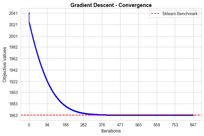
_images/6426bfc0f5a385cd9a88543dc5f760b90e9cd8f421a2bcf1250b90c21df9c8bd.png

Gradient Descent run time: 9.6
Gradient Descent optimal objective: 1863.15
Gradient Descent iterations: 847
Sklearn run time: 0.04
Sklearn optimal objective: 1863.15
Error (divergence): 0.0

The convergence of our Gradient Descent implementation is not good in terms of iterations needed to converge, since it needs 847 iterations, what means 9.6 secs to converge, what is too much in comparison with the sklearn benchmark (0.04 secs). But, in spite of that, the convergence value is basically the benchmark value (null divergence), so, in terms of approximating the optimal of the objective function is pretty good.

Convergence of Coordinate Descent#

start_iter = 240
fig, axes = plt.subplots(1, 2, figsize=(15, 5))
axes = axes.flatten()  
sns.lineplot(y=coordinate_descent.objective_values, 
             x=range(0, coordinate_descent.break_iter), 
             marker='o', markersize=3, color='blue', markeredgewidth=0, ax=axes[0])
sns.lineplot(y=coordinate_descent.objective_values[start_iter:], 
             x=range(start_iter, coordinate_descent.break_iter), 
             marker='o', markersize=3, color='blue', markeredgewidth=0, ax=axes[1])
axes[0].set_title(f'Objective Function vs Iterations', fontsize=13)
axes[1].set_title(f'Objective Function vs Iterations[{start_iter}:]', fontsize=13)
axes[0].set_xlabel('Iterations', fontsize=12)
axes[1].set_xlabel('Iterations', fontsize=12)
axes[0].set_ylabel('Objective values', fontsize=12)
axes[1].set_ylabel('Objective values', fontsize=12)
axes[0].set_xticks(np.unique(np.round(np.linspace(0, coordinate_descent.break_iter, 10))))
axes[1].set_xticks(np.unique(np.round(np.linspace(start_iter, coordinate_descent.break_iter, 10))))
y_ticks_0 = [benchmark_results['sklearn']['fun']-100, benchmark_results['sklearn']['fun']] + list(np.unique(np.round(np.linspace(np.min(coordinate_descent.objective_values), 
                                                                                                                                np.max(coordinate_descent.objective_values), 10))))
axes[0].set_yticks(y_ticks_0)
axes[1].set_yticks(np.unique(np.round(np.linspace(np.min(coordinate_descent.objective_values[start_iter:]), 
                                                  np.max(coordinate_descent.objective_values[start_iter:]), 10))))
axes[0].axhline(y=benchmark_results['sklearn']['fun'], color='r', linestyle='--', label='Sklearn Benchmark')
axes[0].legend()
plt.suptitle('Coordinate Descent - Convergence', fontsize=15, y=0.99, weight='bold', color='black', alpha=1)
plt.subplots_adjust(hspace=1, wspace=0.3) 
plt.show()

print('Coordinate Descent run time:', np.round(coordinate_descent.run_time,2))
print('Coordinate Descent optimal objective:', np.round(coordinate_descent.objective_optimal,2))
print('Coordinate Descent iterations:', coordinate_descent.break_iter)
print('Sklearn run time:', np.round(benchmark_results['sklearn']['time'],2))
print('Sklearn optimal objective:', np.round(benchmark_results['sklearn']['fun'],2))
print('Error (divergence):', np.round(coordinate_descent.objective_optimal - benchmark_results['sklearn']['fun'], 2))

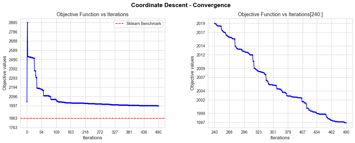
_images/1b4d7192ed34afa839cf3ab3463a2ad7d9db04a181d37924832d4428ec823d31.png

Coordinate Descent run time: 5.55
Coordinate Descent optimal objective: 1996.92
Coordinate Descent iterations: 490
Sklearn run time: 0.04
Sklearn optimal objective: 1863.15
Error (divergence): 133.77

The convergence of our Coordinate Descent implementation is not good in terms of iterations needed to converge, since it needs 490 iterations, what means 5.55 secs to converge, what is too much in comparison with the sklearn benchmark (0.04 secs), but less than with Gradient Descent.

Besides, the convergence value is a bit far from the benchmark value (divergence of 133.77), so, in terms of approximating the optimal of the objective function is not as good as Gradient Descent.

Convergence of Stochastic Gradient Descent#

fig, axes = plt.subplots(figsize=(8, 5))
ax = sns.lineplot(y=stochastic_gradient_descent.objective_values, x=range(0, stochastic_gradient_descent.break_iter), 
             marker='o', markersize=3, color='blue', markeredgewidth=0)
ax.set_title(f'Objective Function vs Iterations', fontsize=13)
ax.set_xlabel('Iterations', fontsize=12)
ax.set_ylabel('Objective values', fontsize=12)
ax.set_xticks(np.unique(np.round(np.linspace(0, stochastic_gradient_descent.break_iter, 10))))
ax.set_yticks(np.unique(np.round(np.linspace(np.min(stochastic_gradient_descent.objective_values), 
                                             np.max(stochastic_gradient_descent.objective_values), 10))))
#ax.axhline(y=benchmark_results['sklearn']['fun'], color='r', linestyle='--', label='Sklearn Benchmark')
plt.title('Stochastic Gradient Descent (Mini-Batch) - Convergence', fontsize=13, y=0.99, weight='bold', color='black', alpha=1)
plt.show()

print('Stochastic Gradient Descent run time:', np.round(stochastic_gradient_descent.run_time,2))
print('Stochastic Descent optimal objective:', np.round(stochastic_gradient_descent.objective_optimal,2))
print('Sklearn run time:', np.round(benchmark_results['sklearn']['time'],2))
print('Sklearn optimal objective:', np.round(benchmark_results['sklearn']['fun'],2))
print('Error (divergence):', np.round(stochastic_gradient_descent.objective_optimal - benchmark_results['sklearn']['fun'], 2))

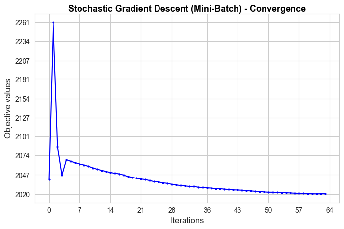
_images/821628f751c8fd8a5cf69fc0a851326863fdf939b90ce4b71c68de339eebba80.png

Stochastic Gradient Descent run time: 0.76
Stochastic Descent optimal objective: 2020.49
Sklearn run time: 0.04
Sklearn optimal objective: 1863.15
Error (divergence): 157.34

The convergence of our Stochastic Gradient Descent (Mini-Batch) implementation is very good in terms of iterations needed to converge, since it needs 64 iterations, what means 0.76 secs to converge, what is more than sklearn benchmark (0.04 secs), but not much more, and quite less than with the previous methods.

Besides, the convergence value is a bit far from the benchmark value (divergence of 157.34), so, in terms of approximating the optimal of the objective function is not as good as above methods.

Convergence of Stochastic Gradient Descent with Momentum#

fig, axes = plt.subplots(figsize=(8, 5))
ax = sns.lineplot(y=stochastic_gradient_descent_momentum.objective_values, x=range(0, stochastic_gradient_descent_momentum.break_iter), 
             marker='o', markersize=3, color='blue', markeredgewidth=0)
ax.set_title(f'Objective Function vs Iterations', fontsize=13)
ax.set_xlabel('Iterations', fontsize=12)
ax.set_ylabel('Objective values', fontsize=12)
ax.set_xticks(np.unique(np.round(np.linspace(0, stochastic_gradient_descent_momentum.break_iter, 10))))
ax.set_yticks(np.unique(np.round(np.linspace(np.min(stochastic_gradient_descent_momentum.objective_values), 
                                             np.max(stochastic_gradient_descent_momentum.objective_values), 10))))
#ax.axhline(y=benchmark_results['sklearn']['fun'], color='r', linestyle='--', label='Sklearn Benchmark')
plt.title('Stochastic Gradient Descent (Mini-Batch) with Momentum - Convergence', fontsize=13, y=0.99, weight='bold', color='black', alpha=1)
plt.show()

print('Stochastic Gradient Descent (momentum) run time:', np.round(stochastic_gradient_descent_momentum.run_time,2))
print('Stochastic Descent (momentum) optimal objective:', np.round(stochastic_gradient_descent_momentum.objective_optimal,2))
print('Sklearn run time:', np.round(benchmark_results['sklearn']['time'],2))
print('Sklearn optimal objective:', np.round(benchmark_results['sklearn']['fun'],2))
print('Error (divergence):', np.round(stochastic_gradient_descent_momentum.objective_optimal - benchmark_results['sklearn']['fun'], 2))

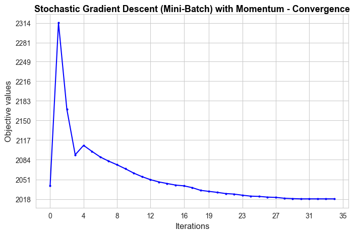
_images/feb271e74f09150e906725b29a1d66154564f82f9824a971d5b4a750e8ddf9d3.png

Stochastic Gradient Descent (momentum) run time: 0.42
Stochastic Descent (momentum) optimal objective: 2018.29
Sklearn run time: 0.04
Sklearn optimal objective: 1863.15
Error (divergence): 155.14

The convergence of our Stochastic Gradient Descent (Mini-Batch) with momentum implementation is good in terms of iterations needed to converge, since it just needs 35 iterations, what means 0.42 secs to converge, what is more than sklearn benchmark (0.04 secs), but not much more, and less than with the previous methods.

Besides, the convergence value is a bit far from the benchmark value (divergence of 155.14), so, in terms of approximating the optimal of the objective function is better than Stochastic Gradient Descent without momentum.

Convergence of Newton’s Method#

fig, axes = plt.subplots(figsize=(8, 5))
ax = sns.lineplot(y=newton.objective_values, x=range(0, newton.break_iter), 
             marker='o', markersize=3, color='blue', markeredgewidth=0)
ax.set_title(f'Objective Function vs Iterations', fontsize=13)
ax.set_xlabel('Iterations', fontsize=12)
ax.set_ylabel('Objective values', fontsize=12)
ax.set_xticks(np.unique(np.round(np.linspace(0, newton.break_iter, 10))))
ax.set_yticks(np.unique(np.round(np.linspace(np.min(newton.objective_values), np.max(newton.objective_values), 10))))
ax.axhline(y=benchmark_results['sklearn']['fun'], color='r', linestyle='--', label='Sklearn Benchmark')
plt.title('Newton\'s Method -  Convergence', fontsize=13, y=0.99, weight='bold', color='black', alpha=1)
plt.legend()
plt.show()

print('Newton\'s Method run time:', np.round(newton.run_time,2))
print('Newton\'s Method optimal objective:', np.round(newton.objective_optimal,2))
print('Sklearn run time:', np.round(benchmark_results['sklearn']['time'],2))
print('Sklearn optimal objective:', np.round(benchmark_results['sklearn']['fun'],2))
print('Error (divergence):', np.round(newton.objective_optimal - benchmark_results['sklearn']['fun'], 2))

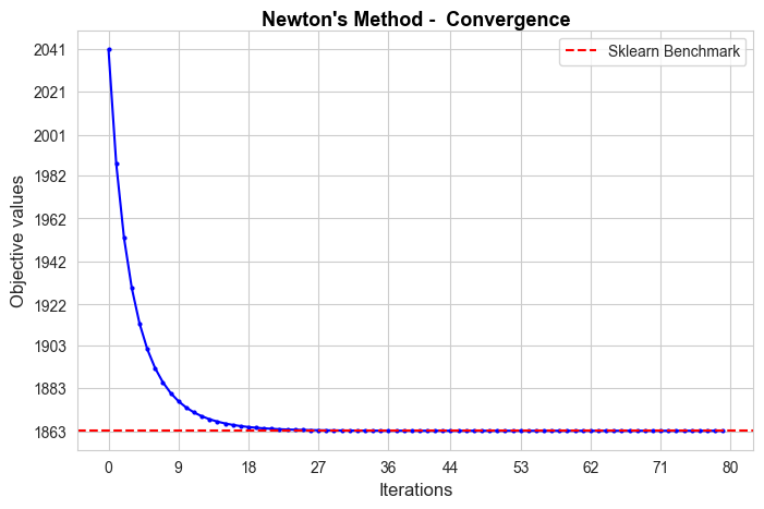
_images/932d7f8a74147f9548dfd601b739db73c217e9a8d9c3b570b295174c6f0677d2.png

Newton's Method run time: 193.38
Newton's Method optimal objective: 1863.15
Sklearn run time: 0.04
Sklearn optimal objective: 1863.15
Error (divergence): 0.0

The convergence of our Newton’s Method implementation is bad in terms of iterations needed to converge, since it needs 80 iterations, what means 193.38 secs to converge, what is much more than sklearn benchmark (0.04 secs), and it’s by far the most expensive method.

But, in spite of that, the convergence value is the same of the benchmark value (null divergence), so, in terms of approximating the optimal of the objective function is brilliant.

Convergence of Stochastic Newton’s Method#

start_iter = 10
fig, axes = plt.subplots(1, 2, figsize=(15, 5))
axes = axes.flatten()  
sns.lineplot(y=stochastic_newton.objective_values, 
             x=range(0, stochastic_newton.break_iter), 
             marker='o', markersize=3, color='blue', markeredgewidth=0, ax=axes[0])
sns.lineplot(y=stochastic_newton.objective_values[start_iter:], 
             x=range(start_iter, stochastic_newton.break_iter), 
             marker='o', markersize=3, color='blue', markeredgewidth=0, ax=axes[1])
axes[0].set_title(f'Objective Function vs Iterations', fontsize=13)
axes[1].set_title(f'Objective Function vs Iterations[{start_iter}:]', fontsize=13)
axes[0].set_xlabel('Iterations', fontsize=12)
axes[1].set_xlabel('Iterations', fontsize=12)
axes[0].set_ylabel('Objective values', fontsize=12)
axes[1].set_ylabel('Objective values', fontsize=12)
axes[0].set_xticks(np.unique(np.round(np.linspace(0, stochastic_newton.break_iter, 10))))
axes[1].set_xticks(np.unique(np.round(np.linspace(start_iter, stochastic_newton.break_iter, 10))))
axes[0].axhline(y=benchmark_results['sklearn']['fun'], color='r', linestyle='--', label='Sklearn Benchmark')
axes[0].legend()
y_ticks_0 = [np.round(benchmark_results['sklearn']['fun'])] + list(np.unique(np.round(np.linspace(np.min(stochastic_newton.objective_values), 
                                                                                                  np.max(stochastic_newton.objective_values), 10))))
axes[0].set_yticks(y_ticks_0)
axes[1].set_yticks(np.unique(np.round(np.linspace(np.min(stochastic_newton.objective_values[start_iter:]), 
                                      np.max(stochastic_newton.objective_values[start_iter:]), 10))))
plt.suptitle('Stochastic Newton\'s Method - Convergence', fontsize=15, y=0.99, weight='bold', color='black', alpha=1)
plt.subplots_adjust(hspace=1, wspace=0.3) 
plt.show()

print('Stochastic Newton\'s Method run time:', np.round(stochastic_newton.run_time,2))
print('Stochastic Newton\'s Method optimal objective:', np.round(stochastic_newton.objective_optimal,2))
print('Sklearn run time:', np.round(benchmark_results['sklearn']['time'],2))
print('Sklearn optimal objective:', np.round(benchmark_results['sklearn']['fun'],2))
print('Error (divergence):', np.round(stochastic_newton.objective_optimal - benchmark_results['sklearn']['fun'], 2))

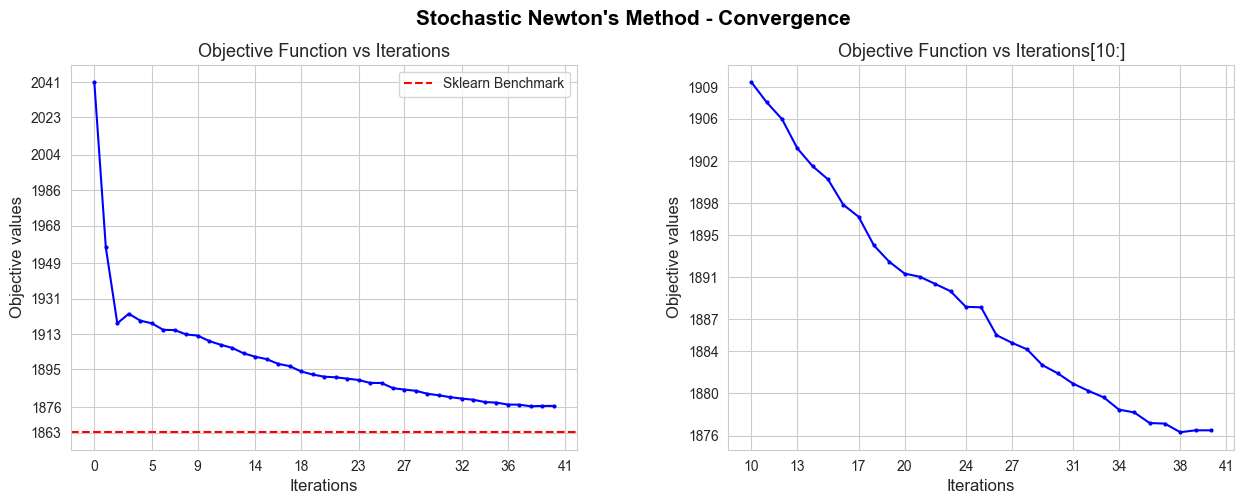
_images/33c9d4b6aef97cd35510114fa63d44194efdf9b23c6efa62bde93a67ce256b95.png

Stochastic Newton's Method run time: 0.84
Stochastic Newton's Method optimal objective: 1876.49
Sklearn run time: 0.04
Sklearn optimal objective: 1863.15
Error (divergence): 13.34

The convergence of our Stochastic Newton’s Method implementation is good in terms of iterations needed to converge, since it needs 41 iterations, what means 0.84 secs to converge, what is more than sklearn benchmark (0.04 secs), but not much.

In addition, the convergence value is close to the benchmark value (13.34 divergence), so, in terms of approximating the optimal of the objective function is pretty good.

This is so far the best of our Stochastic implementations.

Convergence of Quasi-Newton’s BFGS Method#

fig, axes = plt.subplots(figsize=(8, 5))
ax = sns.lineplot(y=quasi_newton_BFGS.objective_values, x=range(0, quasi_newton_BFGS.break_iter), 
             marker='o', markersize=3, color='blue', markeredgewidth=0)
ax.set_title(f'Objective Function vs Iterations', fontsize=13)
ax.set_xlabel('Iterations', fontsize=12)
ax.set_ylabel('Objective values', fontsize=12)
ax.set_xticks(np.unique(np.round(np.linspace(0, quasi_newton_BFGS.break_iter, 10))))
ax.set_yticks(np.unique(np.round(np.linspace(np.min(quasi_newton_BFGS.objective_values), np.max(quasi_newton_BFGS.objective_values), 10))))
ax.axhline(y=benchmark_results['sklearn']['fun'], color='r', linestyle='--', label='Sklearn Benchmark')
plt.title('Quasi-Newton\'s Method BFGS - Convergence', fontsize=13, y=0.99, weight='bold', color='black', alpha=1)
plt.legend()
plt.show()

print('Quasi-Newton\'s BFGS Method run time:', np.round(quasi_newton_BFGS.run_time,2))
print('Quasi-Newton\'s BFGS  optimal objective:', np.round(quasi_newton_BFGS.objective_optimal,2))
print('Sklearn run time:', np.round(benchmark_results['sklearn']['time'],2))
print('Sklearn optimal objective:', np.round(benchmark_results['sklearn']['fun'],2))
print('Error (divergence):', np.round(quasi_newton_BFGS.objective_optimal - benchmark_results['sklearn']['fun'], 2))

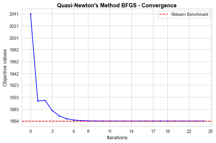
_images/0e0e425be8fe36d145386290003b22b7fc6ea366e55b5d5a1cb8fc13a29e2048.png

Quasi-Newton's BFGS Method run time: 3.06
Quasi-Newton's BFGS  optimal objective: 1863.51
Sklearn run time: 0.04
Sklearn optimal objective: 1863.15
Error (divergence): 0.36

The convergence of our Quasi-Newton’s BFGS Method implementation is good in terms of iterations needed to converge, since it needs 25 iterations, what means 3.06 secs to converge, what is more than sklearn benchmark (0.04 secs), but not too much.

In addition, the convergence value is practically the same of the benchmark value (0.36 divergence), so, in terms of approximating the optimal of the objective function is pretty good.

Convergence of Quasi-Newton’s SR1 Method#

fig, axes = plt.subplots(figsize=(8, 5))
ax = sns.lineplot(y=quasi_newton_SR1.objective_values, x=range(0, quasi_newton_SR1.break_iter), 
             marker='o', markersize=3, color='blue', markeredgewidth=0)
ax.set_title(f'Objective Function vs Iterations', fontsize=13)
ax.set_xlabel('Iterations', fontsize=12)
ax.set_ylabel('Objective values', fontsize=12)
ax.set_xticks(np.unique(np.round(np.linspace(0, quasi_newton_SR1.break_iter, 10))))
ax.set_yticks(np.unique(np.round(np.linspace(np.min(quasi_newton_SR1.objective_values), np.max(quasi_newton_SR1.objective_values), 10))))
ax.axhline(y=benchmark_results['sklearn']['fun'], color='r', linestyle='--', label='Sklearn Benchmark')
plt.title('Quasi Newton\'s SR1 Method - Convergence', fontsize=13, y=0.99, weight='bold', color='black', alpha=1)
plt.legend()
plt.show()

print('Quasi-Newton\'s SR1 Method run time:', np.round(quasi_newton_SR1.run_time,2))
print('Quasi-Newton\'s SR1  optimal objective:', np.round(quasi_newton_SR1.objective_optimal,2))
print('Sklearn run time:', np.round(benchmark_results['sklearn']['time'],2))
print('Sklearn optimal objective:', np.round(benchmark_results['sklearn']['fun'],2))
print('Error (divergence):', np.round(quasi_newton_SR1.objective_optimal - benchmark_results['sklearn']['fun'], 2))

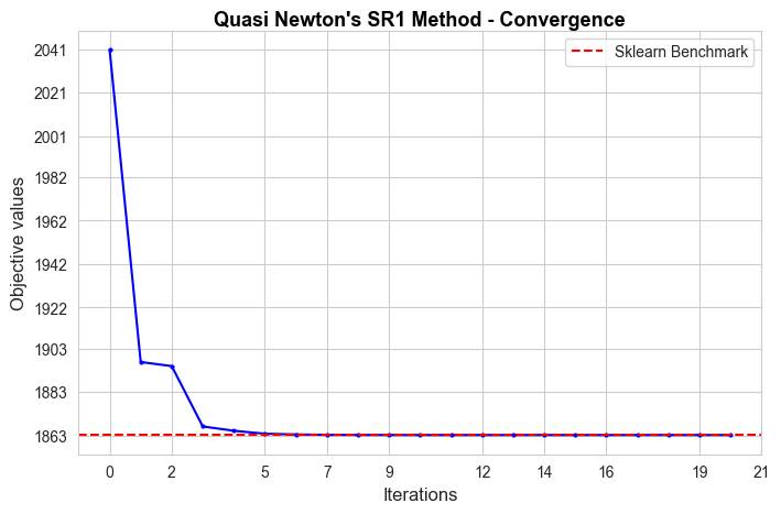
_images/9168618d69fdd9c751eb66c9885b639479eb697432ef4bbc7fbec1427a56908e.png

Quasi-Newton's SR1 Method run time: 3.03
Quasi-Newton's SR1  optimal objective: 1863.15
Sklearn run time: 0.04
Sklearn optimal objective: 1863.15
Error (divergence): 0.0

The convergence of our Quasi-Newton’s SR1 Method implementation is good in terms of iterations needed to converge, since it needs 25 iterations, what means 3.03 secs to converge, what is more than sklearn benchmark (0.04 secs), but not too much.

In addition, the convergence value is the same of the benchmark value (null divergence), so, in terms of approximating the optimal of the objective function is perfect.

Stochastic Convergence of Quasi-Newton’s BFGS Method#

fig, axes = plt.subplots(figsize=(8, 5))
ax = sns.lineplot(y=stochastic_quasi_newton_BFGS.objective_values, x=range(0, stochastic_quasi_newton_BFGS.break_iter), 
             marker='o', markersize=3, color='blue', markeredgewidth=0)
ax.set_title(f'Objective Function vs Iterations', fontsize=13)
ax.set_xlabel('Iterations', fontsize=12)
ax.set_ylabel('Objective values', fontsize=12)
ax.set_xticks(np.unique(np.round(np.linspace(0, stochastic_quasi_newton_BFGS.break_iter, 10))))
ax.set_yticks([np.round(benchmark_results['sklearn']['fun'])-15, np.round(benchmark_results['sklearn']['fun'])] + list(np.unique(np.round(np.linspace(np.min(stochastic_quasi_newton_BFGS.objective_values), 
                                                                                                    np.max(stochastic_quasi_newton_BFGS.objective_values), 10)))))
ax.axhline(y=benchmark_results['sklearn']['fun'], color='r', linestyle='--', label='Sklearn Benchmark')
plt.title('Stochastic Quasi Newton\'s BFGS Method - Convergence', fontsize=13, y=0.99, weight='bold', color='black', alpha=1)
plt.legend()
plt.show()

print('Stochastic Quasi-Newton\'s BFGS Method run time:', np.round(stochastic_quasi_newton_BFGS.run_time,2))
print('Stochastic Quasi-Newton\'s BFGS  optimal objective:', np.round(stochastic_quasi_newton_BFGS.objective_optimal,2))
print('Sklearn run time:', np.round(benchmark_results['sklearn']['time'],2))
print('Sklearn optimal objective:', np.round(benchmark_results['sklearn']['fun'],2))
print('Error (divergence):', np.round(stochastic_quasi_newton_BFGS.objective_optimal - benchmark_results['sklearn']['fun'], 2))

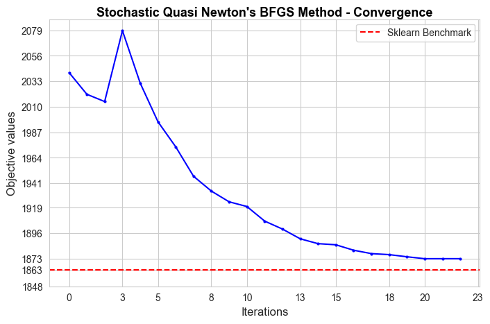
_images/65fe4a37013b16945f8735531a112e48c050054070dec2c572f9b2f12e0ff04e.png

Stochastic Quasi-Newton's BFGS Method run time: 0.54
Stochastic Quasi-Newton's BFGS  optimal objective: 1872.94
Sklearn run time: 0.04
Sklearn optimal objective: 1863.15
Error (divergence): 9.79

The convergence of our Stochastic Quasi-Newton’s BFGS Method implementation is pretty good in terms of iterations needed to converge, since it needs 23 iterations, what means 0.54 secs to converge, what is more than sklearn benchmark (0.04 secs), but not much.

In addition, the convergence value is the close to the benchmark value (9.79 divergence), so, in terms of approximating the optimal of the objective function is good.

Stochastic Convergence of Quasi-Newton’s SR1 Method#

fig, axes = plt.subplots(figsize=(8, 5))
ax = sns.lineplot(y=stochastic_quasi_newton_SR1.objective_values, x=range(0, stochastic_quasi_newton_SR1.break_iter), 
             marker='o', markersize=3, color='blue', markeredgewidth=0)
ax.set_title(f'Objective Function vs Iterations', fontsize=13)
ax.set_xlabel('Iterations', fontsize=12)
ax.set_ylabel('Objective values', fontsize=12)
ax.set_xticks(np.unique(np.round(np.linspace(0, stochastic_quasi_newton_SR1.break_iter, 10))))
ax.set_yticks([np.round(benchmark_results['sklearn']['fun'])-15, np.round(benchmark_results['sklearn']['fun'])] + list(np.unique(np.round(np.linspace(np.min(stochastic_quasi_newton_SR1.objective_values), 
                                                                                                    np.max(stochastic_quasi_newton_SR1.objective_values), 10)))))
ax.axhline(y=benchmark_results['sklearn']['fun'], color='r', linestyle='--', label='Sklearn Benchmark')
plt.title('Stochastic Quasi Newton\'s SR1 Method - Convergence', fontsize=13, y=0.99, weight='bold', color='black', alpha=1)
plt.legend()
plt.show()

print('Stochastic Quasi-Newton\'s SR1 Method run time:', np.round(stochastic_quasi_newton_SR1.run_time,2))
print('Stochastic Quasi-Newton\'s SR1  optimal objective:', np.round(stochastic_quasi_newton_SR1.objective_optimal,2))
print('Sklearn run time:', np.round(benchmark_results['sklearn']['time'],2))
print('Sklearn optimal objective:', np.round(benchmark_results['sklearn']['fun'],2))
print('Error (divergence):', np.round(stochastic_quasi_newton_SR1.objective_optimal - benchmark_results['sklearn']['fun'], 2))

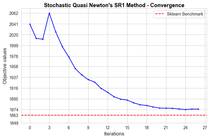
_images/45d3dd58627a1a996d0b3404ac25e199fe59d1f9db1258a77377e260da260993.png

Stochastic Quasi-Newton's SR1 Method run time: 0.34
Stochastic Quasi-Newton's SR1  optimal objective: 1874.85
Sklearn run time: 0.04
Sklearn optimal objective: 1863.15
Error (divergence): 11.71

The convergence of our Stochastic Quasi-Newton’s SR1 Method implementation is pretty good in terms of iterations needed to converge, since it needs 16 iterations, what means 0.34 secs to converge, what is more than sklearn benchmark (0.04 secs), but a bit less than with BFGS rule.

In addition, the convergence value is the close to the benchmark value (11.71 divergence), so, in terms of approximating the optimal of the objective function is good but a bit more than with the BFGS rule.

Methods Comparison: Optimal values vs Times#

In this section we are going to compare all the tested methods (both our implementations and the sklearn and scipy ones) in terms of optimality and time.

methods = {}
methods['gradient_descent'] = gradient_descent
methods['coordinate_descent'] = coordinate_descent
methods['stochastic_gradient_descent'] = stochastic_gradient_descent
methods['stochastic_gradient_descent_momentum'] = stochastic_gradient_descent_momentum
methods['newton'] = newton
methods['stochastic_newton'] = stochastic_newton
methods['quasi_newton_BFGS'] = quasi_newton_BFGS
methods['quasi_newton_SR1'] = quasi_newton_SR1
methods['stochastic_quasi_newton_BFGS'] = stochastic_quasi_newton_BFGS
methods['stochastic_quasi_newton_SR1'] = stochastic_quasi_newton_SR1

methods_list = [x for x in methods.keys()]
optimal_values_methods = [methods[x].objective_optimal for x in methods_list]
times_methods = [methods[x].run_time for x in methods_list]

for method in benchmark_methods:
    methods_list.append(method)
    optimal_values_methods.append(benchmark_results[method]['fun'])
    times_methods.append(benchmark_results[method]['time'])

best_method_objective = methods_list[np.argsort(optimal_values_methods)[0]]
best_objective = np.min(optimal_values_methods)
best_method_time = methods_list[np.argsort(times_methods)[0]]
best_time = np.min(times_methods)
optimal_values_methods = np.array(optimal_values_methods)
times_methods = np.array(times_methods)
error_to_best = np.round(optimal_values_methods - best_objective,2)
time_to_best = np.round(times_methods - best_time,2)
comparison_table = pd.DataFrame({'Method': methods_list, 'Optimality': optimal_values_methods, 'Error': error_to_best, 
                                 'Time': times_methods, 'Time_to_best': time_to_best})

scaler = MinMaxScaler(feature_range=(0,1))
scaler.fit(times_methods.reshape(-1,1))
times_methods_scaled = scaler.transform(times_methods.reshape(-1,1)).flatten()
scaler.fit(optimal_values_methods.reshape(-1,1))
optimal_values_methods_scaled = scaler.transform(optimal_values_methods.reshape(-1,1)).flatten()
best_method_objective_scaled = methods_list[np.argsort(optimal_values_methods_scaled)[0]]
best_objective_scaled = np.min(optimal_values_methods_scaled)
best_method_time_scaled = methods_list[np.argsort(times_methods_scaled)[0]]
best_time_scaled = np.min(times_methods_scaled)

fig, axes = plt.subplots(1, 2, figsize=(10, 5))
axes = axes.flatten()  

sns.scatterplot(x=optimal_values_methods, y=methods_list, marker='*', color='black', s=300, ax=axes[0])
sns.scatterplot(x=[best_objective], y=[best_method_objective], marker='*', color='red', s=300, ax=axes[0])

sns.scatterplot(x=times_methods, y=methods_list, color='blue', s=60, ax=axes[1])
sns.scatterplot(x=[best_time], y=[best_method_time], color='red', s=60, ax=axes[1])

axes[0].set_title(f'Methods vs Objective Function', fontsize=12)
axes[1].set_title(f'Methods vs Time', fontsize=12)
axes[0].set_xlabel('Objective value', fontsize=12)
axes[1].set_xlabel('Time', fontsize=12)
axes[0].set_ylabel('Methods', fontsize=12)
axes[1].yaxis.set_ticklabels([])
#axes[1].set_ylabel('Objective values', fontsize=12)
axes[0].set_xticks(np.round(np.linspace(np.min(optimal_values_methods), np.max(optimal_values_methods), 7)))
axes[1].set_xticks(np.arange(0, np.max(times_methods)+5, 15))
plt.suptitle('Methods Comparison - Optimality and Time', fontsize=15, y=0.99, weight='bold', color='black', alpha=1)
plt.subplots_adjust(hspace=1, wspace=0.05) 
plt.show()

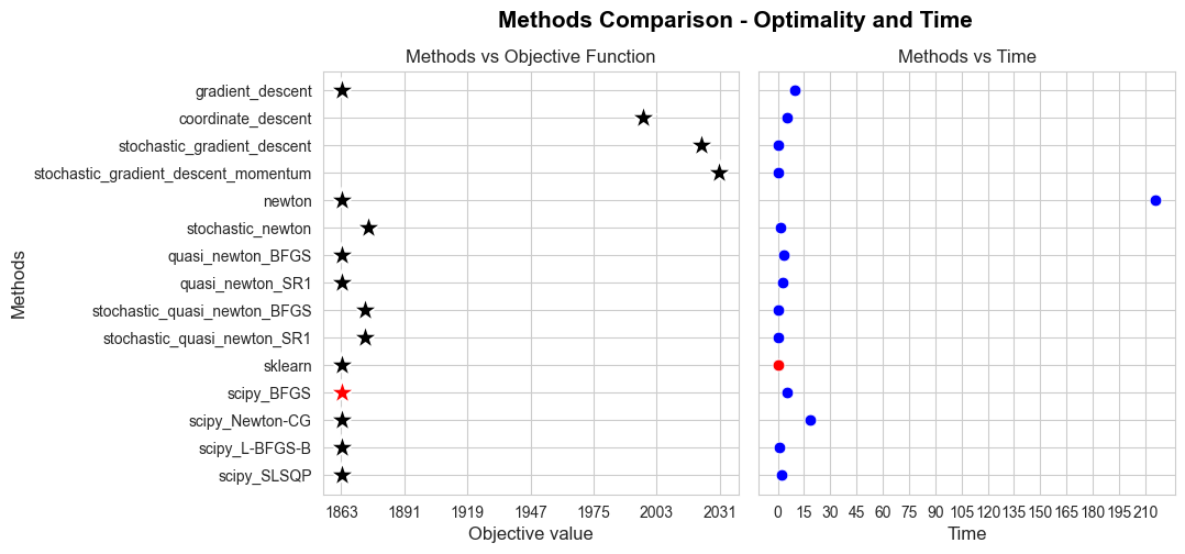
_images/47ab8c2e7bad441a76414ed0caa762a3a1f1a861fb5c8bafb3b1f8e6658bc1a5.png

In order to make a more fruitful comparison we are going to scale the objective and time values, to bring them to the same scale and make them comparable.

fig, axes = plt.subplots(figsize=(5, 5))

ax=sns.scatterplot(x=optimal_values_methods_scaled, y=methods_list,
                marker='*', color='black', s=300, label='Objective value')
ax=sns.scatterplot(x=[best_objective_scaled], y=[best_method_objective_scaled], 
                marker='*', color='red', s=300)

ax=sns.scatterplot(x=times_methods_scaled, y=methods_list, 
                marker='o', color='blue', s=60, label='Time')
ax=sns.scatterplot(x=[best_time_scaled], y=[best_method_time_scaled], 
                marker='o', color='red', s=60)
plt.title('Methods Comparison - Optimality vs Time', fontsize=13, y=0.99, weight='bold', color='black', alpha=1)
ax.set_xlabel('Objective - Time (MinMax Scaled)', fontsize=12)
ax.set_ylabel('Methods', fontsize=12)
plt.legend(loc="upper right", bbox_to_anchor=(1.42, 1.0))
plt.show()

print('Stochastic Quasi-Newton\'s BFGS Method time:', np.round(stochastic_quasi_newton_BFGS.run_time,2))
print('Stochastic Quasi-Newton\'s BFGS  optimal objective:', np.round(stochastic_quasi_newton_BFGS.objective_optimal,2))
print('Sklearn time:', np.round(benchmark_results['sklearn']['time'],2))
print('Sklearn optimal objective:', np.round(benchmark_results['sklearn']['fun'],2))

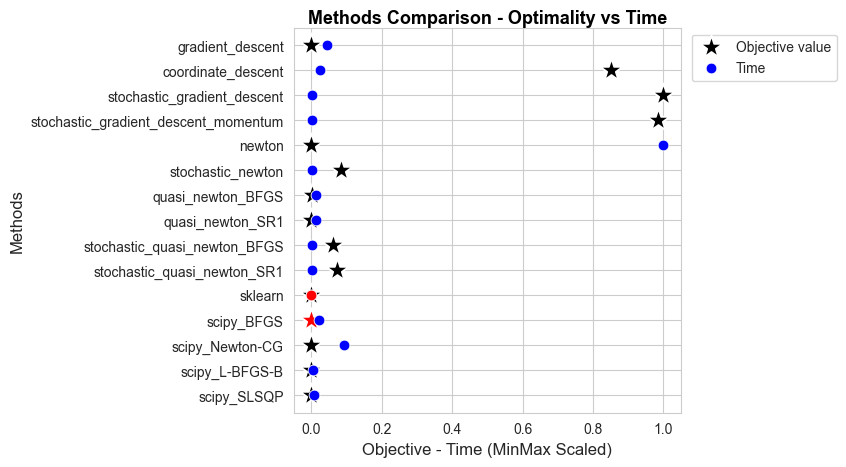
_images/6a51dcbc805c8c35340d08ac9c65b9b6e3fdf74c83ca7b1ed82965e43aaf007f.png

comparison_table.sort_values(by='Error')

	Method	Optimality	Error	Time	Time_to_best
0	gradient_descent	1863.146834	0.00	9.599391	9.56
4	newton	1863.146789	0.00	209.193209	209.15
7	quasi_newton_SR1	1863.148509	0.00	3.032212	2.99
10	sklearn	1863.146785	0.00	0.044000	0.00
11	scipy_BFGS	1863.146785	0.00	4.999240	4.96
12	scipy_Newton-CG	1863.146785	0.00	19.659599	19.62
13	scipy_L-BFGS-B	1863.146785	0.00	0.983402	0.94
14	scipy_SLSQP	1863.146796	0.00	1.614245	1.57
6	quasi_newton_BFGS	1863.508551	0.36	3.060085	3.02
8	stochastic_quasi_newton_BFGS	1872.936608	9.79	0.536080	0.49
9	stochastic_quasi_newton_SR1	1874.854659	11.71	0.341867	0.30
5	stochastic_newton	1876.491136	13.34	0.837814	0.79
1	coordinate_descent	1996.921724	133.77	5.552428	5.51
3	stochastic_gradient_descent_momentum	2018.289185	155.14	0.416592	0.37
2	stochastic_gradient_descent	2020.486231	157.34	0.758967	0.71

comparison_table.sort_values(by='Time')

	Method	Optimality	Error	Time	Time_to_best
10	sklearn	1863.146785	0.00	0.044000	0.00
9	stochastic_quasi_newton_SR1	1874.854659	11.71	0.341867	0.30
3	stochastic_gradient_descent_momentum	2018.289185	155.14	0.416592	0.37
8	stochastic_quasi_newton_BFGS	1872.936608	9.79	0.536080	0.49
2	stochastic_gradient_descent	2020.486231	157.34	0.758967	0.71
5	stochastic_newton	1876.491136	13.34	0.837814	0.79
13	scipy_L-BFGS-B	1863.146785	0.00	0.983402	0.94
14	scipy_SLSQP	1863.146796	0.00	1.614245	1.57
7	quasi_newton_SR1	1863.148509	0.00	3.032212	2.99
6	quasi_newton_BFGS	1863.508551	0.36	3.060085	3.02
11	scipy_BFGS	1863.146785	0.00	4.999240	4.96
1	coordinate_descent	1996.921724	133.77	5.552428	5.51
0	gradient_descent	1863.146834	0.00	9.599391	9.56
12	scipy_Newton-CG	1863.146785	0.00	19.659599	19.62
4	newton	1863.146789	0.00	209.193209	209.15

Some relevant conclusions that we can extract from the above table and plots:

The best methods in terms of optimality are: the sklearn and scipy implementations and our Gradient Descent, Newton and Quasi-Newton SR1 implementations.
The best methods in terms of time are: sklearn is th best, followed by our implementation of Stochastic Quasi-Newton SR1, Stochastic Gradient Descent with momentum and Stochastic Quasi-Newton BFGS.
The best method in terms of trade-off between optimality and time are: sklearn solver, scipy implementation of Quasi-Newton’s L-BFGS-B and SLSQP, followed by our implementations of Quasi-Newton’s BFGS and SR1, and later our Gradient Descent and Stochastic Newton.
- Among our implementations the best is Quasi-Newton’s BFGS and SR1
- Among our stochastic implementations the best is Stochastic Quasi-Newton’s BFGS Method.

Analysis of the sample size effect in some of the stochastic methods#

In this section we are going to explore the effect of the sample size in the stochastic methods (or at least in some of them).

Stochastic Gradient Descent#

sample_size_grid = np.arange(50, 10000, 100)
param_grid = {'sample_size': sample_size_grid}

stochastic_gradient_descent = stochastic_gradient_descent_method(objective=minus_logL, gradient=gradient_function, x_0=initial_betas, 
                                                                 n_iter=2000, tol=1e-6, seed=123, momentum=False)
stochastic_gradient_descent.set_params(**stochastic_gradient_descent_best_params)
random_search = RandomSearch(estimator=stochastic_gradient_descent, param_grid=param_grid, n_trials=len(sample_size_grid), seed=123)
random_search.fit(args=(X,Y))
sgd_sample_size_results = random_search.results

sgd_sample_size_results.head(5)

	sample_size	objective_value	time
22	9750	2016.575250	1.924896
77	9650	2016.707930	1.968579
60	9550	2016.948602	2.532017
12	9950	2017.999126	0.991965
4	9850	2018.105974	0.876709

sgd_sample_size_results.tail(5)

	sample_size	objective_value	time
2	1150	2071.985893	0.330054
72	1550	2074.434644	0.638791
33	1650	2079.663950	1.353488
79	1250	2082.915842	0.802284
5	1350	2085.161451	0.539797

fig, axes = plt.subplots(1, 2, figsize=(12, 5))
axes = axes.flatten()  

sns.scatterplot(x=sgd_sample_size_results['objective_value'], y=sgd_sample_size_results['sample_size'], 
                marker='o', color='black', s=45, ax=axes[0])
sns.scatterplot(x=sgd_sample_size_results['time'], y=sgd_sample_size_results['sample_size'],
                 color='blue', s=45, ax=axes[1])

axes[0].set_title(f'Sample Size vs Objective Function', fontsize=12)
axes[1].set_title(f'Sample Size vs Time', fontsize=12)
axes[0].set_xlabel('Objective value', fontsize=12)
axes[1].set_xlabel('Time (secs)', fontsize=12)
axes[0].set_ylabel('Sample Size', fontsize=12)
axes[1].yaxis.set_ticklabels([])
axes[1].set_ylabel(' ', fontsize=12)
#axes[0].set_xticks(np.round(np.linspace(np.min(sgd_sample_size_results['objective_value']), np.max(sgd_sample_size_results['objective_value']), 7)))
axes[0].set_yticks(np.arange(0, np.max(sgd_sample_size_results['sample_size'])+1000, 800))
axes[0].set_xticks(np.round(np.arange(np.min(sgd_sample_size_results['objective_value']), 
                             np.max(sgd_sample_size_results['objective_value'])+5, 10)))
axes[1].set_yticks(np.arange(0, np.max(sgd_sample_size_results['sample_size'])+1000, 800))
axes[1].set_xticks(np.arange(0, np.max(sgd_sample_size_results['time']+1), 1))
plt.suptitle('Stochastic Gradient Descent - Sample Size Comparison - Optimality and Time', 
             fontsize=15, y=0.99, weight='bold', color='black', alpha=1)
plt.subplots_adjust(hspace=1, wspace=0.05) 
plt.show()

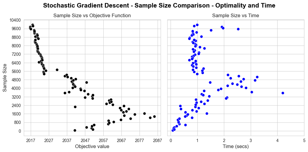
_images/d5e31219f66fb1a8387aebc739246b717e3d889c5fb44b2236109dfe6708186a.png

Some conclusion that can be obtained from the plot:

It seems to be a negative relation between the sample size and the objective value. In general, if a greater sample sized is used to estimate the gradient, a better (lower in this case) objective value is found. But there are some small sample sizes (50-800) that work much better than other larger (1000-3000).
It seems to be a positive relation between the sample size and the computational time, but only for not large enough samples (50-5500). For large enough (5500-10000) the computational time is quite similar (has low variance) and is in average lower than the one of some smaller samples (3200-5000).

Stochastic Newton’s Method#

sn_sample_size_objective_values = []
sn_sample_size_times = []
grad_sample_size_grid = [500, 500, 700, 1000, 1000, 1500, 2000, 2000, 2500, 3000, 4000, 5000, 6000, 3000, 5000, 5000, 6000, 8000]
hess_sample_size_grid = [300, 500, 500, 500,  700, 700, 700, 1000, 1000, 1000, 1000, 1000, 1000, 2000, 2000, 3000, 3000, 5000]

for x,y in zip(grad_sample_size_grid, hess_sample_size_grid):

    stochastic_newton = Stochastic_Newton_method(objective=minus_logL, gradient=gradient_function, hessian=hessian_function, 
                                             x_0=initial_betas, n_iter=2000, tol=1e-6, seed=123, 
                                             grad_sample_size=x, hess_sample_size=y)
    stochastic_newton.set_params(**stochastic_newton_best_params)
    stochastic_newton.fit(args=(X,Y))
    sn_sample_size_objective_values.append(stochastic_newton.objective_optimal)
    sn_sample_size_times.append(stochastic_newton.run_time)

sample_sizes = list(zip(grad_sample_size_grid, hess_sample_size_grid))
sample_sizes = [str(x) for x in sample_sizes]

fig, axes = plt.subplots(1, 2, figsize=(12, 5))
axes = axes.flatten()  

sns.scatterplot(x=sn_sample_size_objective_values, y=sample_sizes, 
                marker='o', color='black', s=60, ax=axes[0])
sns.scatterplot(x=sn_sample_size_times, y=sample_sizes,
                 color='blue', s=60, ax=axes[1])

axes[0].set_title(f'Sample Size vs Objective Function', fontsize=12)
axes[1].set_title(f'Sample Size vs Time', fontsize=12)
axes[0].set_xlabel('Objective value', fontsize=12)
axes[1].set_xlabel('Time (secs)', fontsize=12)
axes[0].set_ylabel('Sample Size', fontsize=12)
axes[1].yaxis.set_ticklabels([])
axes[1].set_ylabel(' ', fontsize=12)
#axes[0].set_xticks(np.round(np.linspace(np.min(sgd_sample_size_results['objective_value']), np.max(sgd_sample_size_results['objective_value']), 7)))
#axes[0].set_yticks(np.arange(0, np.max(sgd_sample_size_results['sample_size'])+1000, 1000))
axes[0].set_xticks(np.round(np.arange(np.min(sn_sample_size_objective_values), 
                             np.max(sn_sample_size_objective_values)+20, 20)))
axes[1].set_xticks(np.arange(0, np.max(sn_sample_size_times)+1, 1))
plt.suptitle('Stochastic Gradient Descent - Sample Size Comparison - Optimality and Time', 
             fontsize=15, y=0.99, weight='bold', color='black', alpha=1)
plt.subplots_adjust(hspace=1, wspace=0.05) 
plt.show()

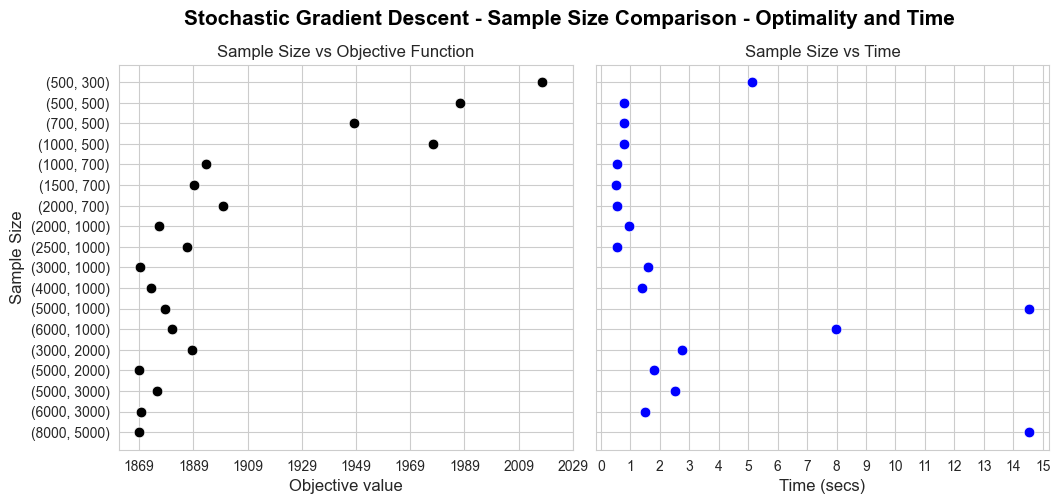
_images/93e1b3372cc7126ed67ca3e7d5a06476f3872c854b7f29661e223cd2423ce178.png

Some conclusions from the plot:

When the combination of sample sizes used to estimated the gradient and the hessian, respectively, is large, the objective value is better (lower in this case).
There seem not to be a clear pattern that govern the relationship between this pairs of sample sizes and the computational time.

Optimizing Penalized Logistic Regression#

In this section we are going to address penalized logistic regression, which is a variant of logistic regression that penalized the betas, enforcing them to fulfill some constraint.

The classic (Ridge) constraint is $|| \beta ||_2^2 = \sum_{j=0}^p \beta_j^2 = 0$ and the idea is to bring some of the coefficient (betas) to zero, in order to add a sort of automatic feature selection to the model.

This is a popular idea in modern statistical learning. Ridge, Lasso and Elastic Net Regression are the greatest exponents of this technique, but it has been exported to other models, like Logistic Regression.

The problem to solve in this section is the following constrained problem:

\[\begin{split}\widehat{\beta} \hspace{0.1cm} = \hspace{0.1cm} arg \hspace{0.1cm} \underset{\beta}{Max} \hspace{0.1cm} log(\mathcal{L}(\beta)) \\[0.3cm] s.t.: \hspace{0.15cm}\small{\sum_{j=0}^p \beta_j^2 = 100}\end{split}\]

Which can be expressed as an unconstrained problem as follows:

\[\widehat{\beta} \hspace{0.1cm} = \hspace{0.1cm} arg \hspace{0.1cm} \underset{\beta}{Min} \hspace{0.1cm} - \Big[\hspace{0.08cm} log(\mathcal{L}(\beta)) - \lambda\cdot \small{\Big(\sum_{j=0}^p \beta_j^2 -100\Big)^2} \hspace{0.08cm}\Big]\]

Applying the conversion to Min problem and the matrix form, we have the following equivalent problem:

\[\widehat{\beta} \hspace{0.1cm} = \hspace{0.1cm} arg \hspace{0.1cm} \underset{\beta}{Min} \hspace{0.1cm} -\Big[\hspace{0.05cm} Y \cdot log(P_1) + (1-Y)\cdot log(1-P_1) \hspace{0.05cm} - \lambda\cdot (\beta^2 - 100)^2\Big]\]

The gradient of $f(\beta)$ is:

\[\nabla f(\beta) \hspace{0.06cm} = \hspace{0.06cm} X^\prime \cdot (P_1-Y) + 2\lambda\cdot (\beta^2 - 100)\cdot 2\beta\]

The hessian of $f(\beta) = - log(\mathcal{L}(\beta))$ is:

\[\nabla^2 f(\beta) \hspace{0.06cm} = \hspace{0.06cm} X^\prime \cdot D \cdot X + 2\lambda \cdot 2 I_p\]

where:

\[D= diag(P_1\cdot (1-P_1))\]

Initial elements#

As we did before, we define the initial elements to address the problem computationally.

def minus_logL_penalized(betas, *args):
    X, Y, pen_lambda = args
    epsilon = 1e-15
    p1 = logistic(X @ betas) 
    sum1 = Y @ np.log(p1 + epsilon)
    sum2 = (1-Y)  @ np.log(1-p1 + epsilon)
    penalization = pen_lambda*(np.sum(betas**2) - 100)**2
    result = - (sum1 + sum2 - penalization)
    return result

def gradient_function_penalized(betas, *args):
    X, Y, pen_lambda = args
    p1 = logistic(X @ betas) 
    gradient = X.T @ (p1 - Y) + 2*pen_lambda*(np.sum(betas**2) - 100)*(2*betas)
    return gradient

def hessian_function_penalized(betas, *args):
    X, Y, pen_lambda = args
    p = X.shape[1]
    p1 = logistic(X @ betas) 
    D = np.diag(p1 * (1 - p1))
    hessian = X.T @ D @ X + (2*pen_lambda)*2*np.identity(p)
    return hessian

pen_lambda = 1 # in (0.7, 2) is enough.

`Sklearn` and `Scipy` optimization#

As before, we will first solve the problem with Scipy solvers.

benchmark_results = {}
benchmark_methods = ['scipy_BFGS', 'scipy_Newton-CG', 'scipy_L-BFGS-B', 'scipy_SLSQP']

# BFGS := Broyden–Fletcher–Goldfarb–Shanno algorithm
# Newton-CG := Newton Conjugate Gradient algorithm
# L-BFGS-B := Limited memory BFGS
# SLSQP := Sequential Least Squares Programming 

for method in benchmark_methods:

    start_time = time.time()
    if method == 'scipy_Newton-CG':
        benchmark_results[method] = minimize(fun=minus_logL_penalized, x0=initial_betas, method=method.split('_')[1], 
                                             jac=gradient_function_penalized, hess=hessian_function_penalized, args=(X,Y,pen_lambda))

    else:
        benchmark_results[method] = minimize(fun=minus_logL_penalized, x0=initial_betas, method=method.split('_')[1], args=(X,Y, pen_lambda))
    end_time = time.time()
    benchmark_results[method]['time'] = end_time - start_time

# Time: 

benchmark_results['scipy_BFGS']

  message: Desired error not necessarily achieved due to precision loss.
  success: False
   status: 2
      fun: 2384.0578128540274
        x: [ 2.541e+00  2.550e+00 ...  6.324e-01  9.169e-01]
      nit: 56
      jac: [ 9.155e-05  9.155e-05 ... -3.052e-05  6.104e-05]
 hess_inv: [[ 7.753e-04  7.914e-05 ...  7.503e-05  1.077e-04]
            [ 7.914e-05  6.824e-04 ...  5.427e-05  1.858e-05]
            ...
            [ 7.503e-05  5.427e-05 ...  6.907e-04  3.014e-05]
            [ 1.077e-04  1.858e-05 ...  3.014e-05  7.279e-04]]
     nfev: 3493
     njev: 129
     time: 8.339475631713867

benchmark_results['scipy_Newton-CG']

 message: Optimization terminated successfully.
 success: True
  status: 0
     fun: 2384.0578133289528
       x: [ 2.541e+00  2.550e+00 ...  6.324e-01  9.168e-01]
     nit: 9
     jac: [ 4.150e-02 -3.019e-02 ... -2.178e-02 -3.583e-03]
    nfev: 16
    njev: 16
    nhev: 9
    time: 32.1147027015686

benchmark_results['scipy_L-BFGS-B']

  message: CONVERGENCE: REL_REDUCTION_OF_F_<=_FACTR*EPSMCH
  success: True
   status: 0
      fun: 2384.0578128542115
        x: [ 2.541e+00  2.550e+00 ...  6.324e-01  9.169e-01]
      nit: 11
      jac: [ 1.364e-04  1.364e-04 ...  0.000e+00  3.183e-04]
     nfev: 351
     njev: 13
 hess_inv: <26x26 LbfgsInvHessProduct with dtype=float64>
     time: 1.153794765472412

benchmark_results['scipy_SLSQP']

 message: Optimization terminated successfully
 success: True
  status: 0
     fun: 2384.057813545238
       x: [ 2.541e+00  2.550e+00 ...  6.324e-01  9.169e-01]
     nit: 25
     jac: [-1.343e-03 -5.524e-03 ...  6.500e-03  1.306e-02]
    nfev: 737
    njev: 25
    time: 1.7633354663848877

We can check easily if the constraint is fulfilled:

np.sum(benchmark_results['scipy_BFGS'].x**2)

103.45900689903829

np.sum(benchmark_results['scipy_Newton-CG'].x**2)

103.45907721935968

np.sum(benchmark_results['scipy_L-BFGS-B'].x**2)

103.45900666588769

np.sum(benchmark_results['scipy_SLSQP'].x**2)

103.45905741002673

We can see that with $\lambda =1$ constraint not totally satisfy, but is close to it.

HPO#

In this section we are going to solve the new problem only with one of our implemented methods, for the shake of brevity.

The chosen method is the Stochastic Quasi-Newton BFGS Method, which was the best among our Stochastic implementations in the previous section.

pen_lambda = 1
learning_rate_grid = np.logspace(-4, -3, num=55)
phi_grid = np.arange(0.1, 1, 0.01)
#sigma_grid = np.logspace(-2, -1, num=50)
param_grid = {'learning_rate': learning_rate_grid, 'phi': phi_grid}

stochastic_quasi_newton_BFGS = Stochastic_Quasi_Newton_method(objective=minus_logL_penalized, gradient=gradient_function_penalized, hessian=hessian_function_penalized, 
                                                              x_0=initial_betas, n_iter=2000, tol=1e-6, grad_sample_size=2000, hess_sample_size=1000, seed=123, rule='BFGS')

random_search = RandomSearch(estimator=stochastic_quasi_newton_BFGS, param_grid=param_grid, n_trials=50, seed=123)
random_search.fit(args=(X,Y, pen_lambda))
stochastic_quasi_newton_BFGS_penalized_best_params = random_search.best_params_
stochastic_quasi_newton_BFGS_penalized_results = random_search.results

C:\Users\fscielzo\AppData\Local\Temp\ipykernel_4396\3752159407.py:74: RuntimeWarning: invalid value encountered in scalar divide
  B[k+1] = B[k] - (M1 @ M1.T)/M2 + M3/M4

stochastic_quasi_newton_BFGS_penalized_results.head(10)

	learning_rate	phi	objective_value	time
8	0.000774	0.82	2414.395541	3.294048
44	0.000742	0.53	2435.829487	0.134308
47	0.000742	0.97	2437.416647	0.796468
38	0.000626	0.46	2453.170528	0.567720
45	0.000626	0.96	2453.426843	0.834335
40	0.000599	0.74	2471.449251	0.648206
48	0.000880	0.46	2474.771527	6.856022
9	0.000880	0.26	2474.771527	3.889722
16	0.000880	0.15	2474.771527	4.042038
37	0.000918	0.27	2513.489051	4.228621

The penalty seems to affect the calculation time, increasing it.

stochastic_quasi_newton_BFGS_penalized_results['time'].mean()

1.899277400970459

stochastic_quasi_newton_BFGS_results['time'].mean()

2.3946699798107147

We fit the method with the best parameters find during the HPO phase.

stochastic_quasi_newton_BFGS_penalized = Stochastic_Quasi_Newton_method(objective=minus_logL_penalized, gradient=gradient_function_penalized, hessian=hessian_function_penalized, 
                                                   x_0=initial_betas, n_iter=2000, tol=1e-6, grad_sample_size=2000, hess_sample_size=1000, seed=123, rule='BFGS')
stochastic_quasi_newton_BFGS_penalized.set_params(**stochastic_quasi_newton_BFGS_penalized_best_params)
stochastic_quasi_newton_BFGS_penalized.fit(args=(X,Y, pen_lambda))

stochastic_quasi_newton_BFGS_penalized.objective_optimal

2414.3955411016636

stochastic_quasi_newton_BFGS_penalized.x_optimal

array([ 2.49175735,  2.48437229,  2.47435553, -0.02026137, -2.56829027,
       -1.23482926, -2.83378562,  1.23127567, -3.08038169,  2.84108034,
        2.18704128,  1.53785186,  0.32576063, -1.55905894,  0.5476085 ,
        0.57765483, -0.29964037, -3.0904155 ,  1.56870018, -2.21738445,
       -3.12750058,  2.17646045,  1.83412108, -0.33615271,  0.63636938,
        0.87384157])

stochastic_quasi_newton_BFGS_penalized.break_iter

We can check if the constrain is fulfilled.

np.sum(stochastic_quasi_newton_BFGS_penalized.x_optimal**2)

100.23194704760508

Analysis of lambda influence in the constraint compliance#

reached_constraint_values, reached_constraint_times = [], []
pen_lambda_grid = [0.3, 0.5, 0.7, 1, 2, 3, 4, 5, 7, 10, 15, 20, 30, 50, 70, 90, 100, 130, 170, 200, 300, 400, 700, 1000]

for pen_lambda in pen_lambda_grid:
    stochastic_quasi_newton_BFGS_penalized.fit(args=(X,Y, pen_lambda))
    reached_constraint_values.append(np.sum(stochastic_quasi_newton_BFGS_penalized.x_optimal**2))
    reached_constraint_times.append(stochastic_quasi_newton_BFGS_penalized.run_time)

fig, axes = plt.subplots(1, 2, figsize=(15, 5))
axes = axes.flatten()  

ax = sns.lineplot(y=reached_constraint_values, x=pen_lambda_grid, ax=axes[0],
                  marker='o', markersize=5, color='black', markeredgewidth=0)
ax = sns.lineplot(y=reached_constraint_times, x=pen_lambda_grid, ax=axes[1],
                  marker='o', markersize=5, color='blue', markeredgewidth=0)
axes[0].set_title(f'Constraint value vs $\\lambda$', fontsize=12)
axes[1].set_title(f'Time vs $\\lambda$', fontsize=12)
axes[0].set_xlabel('$\\lambda$', fontsize=12)
axes[1].set_xlabel('$\\lambda$', fontsize=12)
axes[0].set_ylabel('Constraint value', fontsize=12)
axes[1].set_ylabel('Time (secs)', fontsize=12)
axes[0].axhline(y=100, color='r', linestyle='--', label='True Constraint')
axes[0].set_xticks(np.arange(0, np.max(pen_lambda_grid)+50, 100))
axes[1].set_xticks(np.arange(0, np.max(pen_lambda_grid)+50, 100))
plt.suptitle('Stochastic Newton\'s Method - Penalization Parameter - Reached Constraint and Time', 
             fontsize=15, y=0.99, weight='bold', color='black', alpha=1)
axes[0].legend()
plt.subplots_adjust(hspace=1, wspace=0.3) 
plt.show()

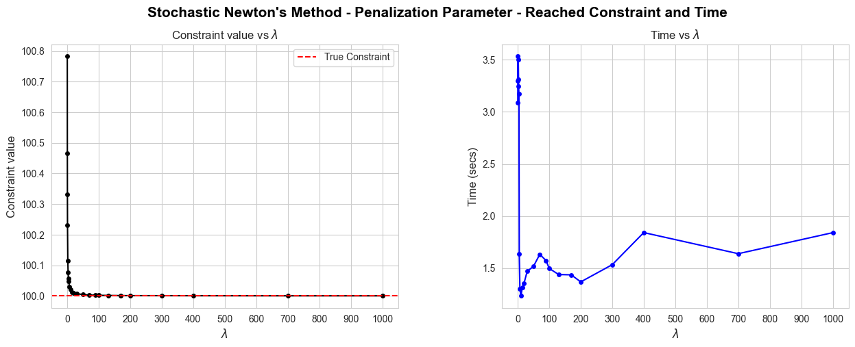
_images/855c3432d89f17783416e9628bffd438d9bc4c1bd0087086c49f8539a9c10107.png

zoom_limit = 12
fig, axes = plt.subplots(1, 2, figsize=(15, 5))
axes = axes.flatten()  

ax = sns.lineplot(y=reached_constraint_values[0:zoom_limit], x=pen_lambda_grid[0:zoom_limit], ax=axes[0],
                  marker='o', markersize=5, color='black', markeredgewidth=0)
ax = sns.lineplot(y=reached_constraint_times[0:zoom_limit], x=pen_lambda_grid[0:zoom_limit], ax=axes[1],
                  marker='o', markersize=5, color='blue', markeredgewidth=0)
axes[0].set_title(f'Constraint value vs $\\lambda$', fontsize=12)
axes[1].set_title(f'Time vs $\\lambda$', fontsize=12)
axes[0].set_xlabel('$\\lambda$', fontsize=12)
axes[1].set_xlabel('$\\lambda$', fontsize=12)
axes[0].set_ylabel('Constraint value', fontsize=12)
axes[1].set_ylabel('Time (secs)', fontsize=12)
axes[0].axhline(y=100, color='r', linestyle='--', label='True Constraint')
axes[0].set_yticks(np.round(np.arange(np.min(reached_constraint_values[0:zoom_limit]), 
                                      np.max(reached_constraint_values[0:zoom_limit])+0.1, 0.1),1))
axes[0].set_xticks(np.arange(0, np.max(pen_lambda_grid[0:zoom_limit])+1, 4))
axes[1].set_xticks(np.arange(0, np.max(pen_lambda_grid[0:zoom_limit])+1, 4))
plt.suptitle('Zoom - Stochastic Newton\'s Method - Penalization Parameter - Reached Constraint and Time', 
             fontsize=15, y=0.99, weight='bold', color='black', alpha=1)
axes[0].legend()
plt.subplots_adjust(hspace=1, wspace=0.3) 
plt.show()

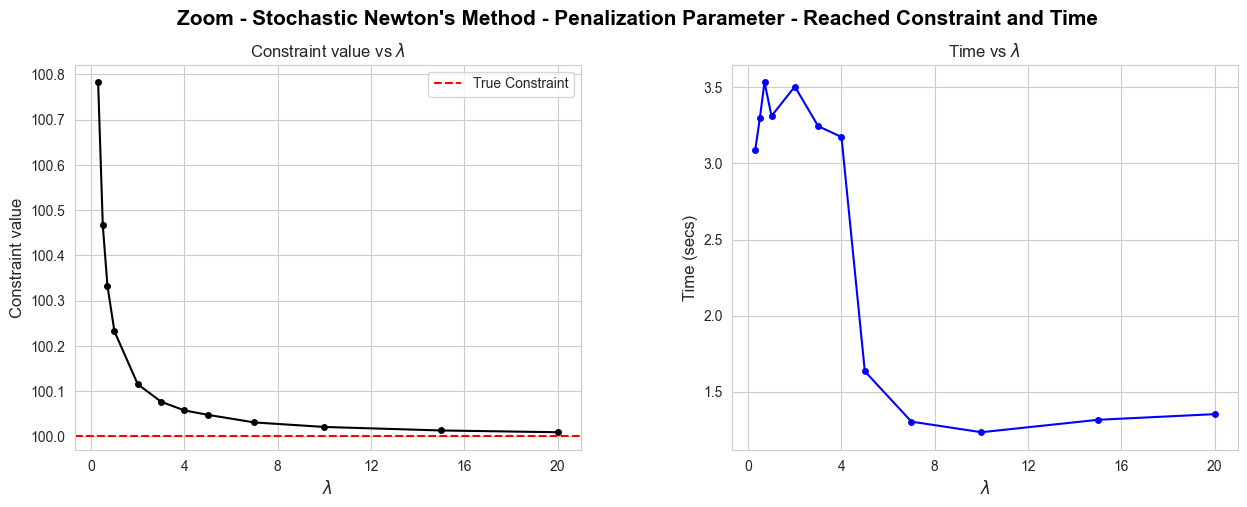
_images/7d55b44adc74928011173a1c71f323c11c108da29a99c64c2332836f025aef03.png

Conclusions:

When $\lambda$ is in $(0,4]$ the convergence is slower than when is $> 4$, even for large values of lambda, such as $1000$.
For $\lambda >= 3$ the difference between the reached constraint and the tue is less than $0.1$. And for $\lambda >7$ there are non significative differences, in other words, the constraint is satisfy.
Even for small $\lambda$ like $0.5$, $0.7$ and $1$, the constraint is almost fulfilled (the difference is less than $0.5$).

Numerical Optimization applied to Logistic Regression

Contents

Numerical Optimization applied to Logistic Regression#

Requirements#

Binary Logistic Regression#

Framework#

How to define \(P_r(x_i)\) ?#

Naive approach: Linear Regression#

Logistic Regression approach#

Model estimation#

Model predictions#

Predicting \(P_r(x_i)\)#

Predicting \(\mathcal{Y}\)#

The optimization problem to solve#

Numerical optimization algorithms#

Framework#

Optimality conditions#

Local and Global solutions#

Most important Numerical Optimization algorithms#

Optimizing Logistic Regression#

Initial elements#

Sklearn and Scipy optimization#

Self-implementation of numerical optimization algorithms#

Gradient Descent Method#

Coordinate Descent Method#

Stochastic Gradient Descent (Mini-Batch)#

Newton Method#

Stochastic Newton Method#

Quasi-Newton Method#

Stochastic Quasi-Newton Method#

Hyper-parameters Optimization (HPO)#

HPO for Gradient Descent#

HPO for Stochastic Gradient Descent (Mini-Batch)#

HPO for Coordinate Descent#

HPO for Stochastic Newton#

HPO for Quasi Newton#

HPO for Stochastic Quasi Newton#

Analysis of convergence#

Convergence of Gradient Descent#

Convergence of Coordinate Descent#

Convergence of Stochastic Gradient Descent#

Convergence of Stochastic Gradient Descent with Momentum#

Convergence of Newton’s Method#

Convergence of Stochastic Newton’s Method#

Convergence of Quasi-Newton’s BFGS Method#

Convergence of Quasi-Newton’s SR1 Method#

Stochastic Convergence of Quasi-Newton’s BFGS Method#

Stochastic Convergence of Quasi-Newton’s SR1 Method#

Methods Comparison: Optimal values vs Times#

Analysis of the sample size effect in some of the stochastic methods#

Stochastic Gradient Descent#

Stochastic Newton’s Method#

Optimizing Penalized Logistic Regression#

Initial elements#

Sklearn and Scipy optimization#

HPO#

Analysis of lambda influence in the constraint compliance#

`Sklearn` and `Scipy` optimization#

`Sklearn` and `Scipy` optimization#