Spark vs Pandas vs Polars: time analysis

Introduction

In this project we have carried out three studies on the data provided in a CSV file with information about taxi trips in New York. We have had to clean the dataset first to remove the records with wrong data and remove outliers. To carry out the studies, as it was required, we have used the entire Spark’s API, including the manipulation of RDDs, dataframes and direct SQL. We have also analyzed both execution time and speedup in each study, for doing this we have measure time of the actions in each process, excluding the previous transformations as they are included in the action.

The three studies are the following:

1. Average speed of taxis in terms of the hour: we have done five versions of this study with Spark df, Spark rdd, Spark SQL, Pandas and Polars.

2. Most common taxi trips: Spark df.

3. Average of tips for each zone: Spark SQL.

Requirements

# pip install findspark

We start the Spark Session with all the cores of our computer and divide the tasks with coalesce(32). However, we have perform different tests on the processes using different number of cores.

import findspark
findspark.init()

from pyspark.sql import SparkSession

spark = SparkSession.builder.appName('Intro to Spark').master("local[*]").getOrCreate()
sc = spark.sparkContext

#############################################

import pandas as pd
import numpy as np
import time
import seaborn as sns
import matplotlib.pyplot as plt
sns.set_style("whitegrid")
from pyspark.sql.functions import round, expr, from_unixtime, unix_timestamp, date_format, count, concat, lit, col
from pyspark.sql.types import IntegerType

Next, we read the dataset provided.

taxis_df = spark.read.format("csv").option("inferSchema", "true").option("timestampFormat","yyyy-MM-dd HH:mm:ss").option("header", "true").option("mode", "DROPMALFORMED").load(r"./Data/taxis.csv")
taxis_df = taxis_df.coalesce(32)
taxis_df.show(5)

+--------+--------------------+---------------------+---------------+-------------+----------+------------------+------------+------------+------------+-----------+-----+-------+----------+------------+---------------------+------------+
|VendorID|tpep_pickup_datetime|tpep_dropoff_datetime|passenger_count|trip_distance|RatecodeID|store_and_fwd_flag|PULocationID|DOLocationID|payment_type|fare_amount|extra|mta_tax|tip_amount|tolls_amount|improvement_surcharge|total_amount|
+--------+--------------------+---------------------+---------------+-------------+----------+------------------+------------+------------+------------+-----------+-----+-------+----------+------------+---------------------+------------+
|       1| 2017-01-09 11:13:28|  2017-01-09 11:25:45|              1|          3.3|         1|                 N|         263|         161|           1|       12.5|  0.0|    0.5|       2.0|         0.0|                  0.3|        15.3|
|       1| 2017-01-09 11:32:27|  2017-01-09 11:36:01|              1|          0.9|         1|                 N|         186|         234|           1|        5.0|  0.0|    0.5|      1.45|         0.0|                  0.3|        7.25|
|       1| 2017-01-09 11:38:20|  2017-01-09 11:42:05|              1|          1.1|         1|                 N|         164|         161|           1|        5.5|  0.0|    0.5|       1.0|         0.0|                  0.3|         7.3|
|       1| 2017-01-09 11:52:13|  2017-01-09 11:57:36|              1|          1.1|         1|                 N|         236|          75|           1|        6.0|  0.0|    0.5|       1.7|         0.0|                  0.3|         8.5|
|       2| 2017-01-01 00:00:00|  2017-01-01 00:00:00|              1|         0.02|         2|                 N|         249|         234|           2|       52.0|  0.0|    0.5|       0.0|         0.0|                  0.3|        52.8|
+--------+--------------------+---------------------+---------------+-------------+----------+------------------+------------+------------+------------+-----------+-----+-------+----------+------------+---------------------+------------+
only showing top 5 rows

taxis_df.describe().show()

+-------+-------------------+------------------+------------------+-------------------+------------------+------------------+-----------------+------------------+-----------------+-------------------+-------------------+------------------+-------------------+---------------------+------------------+
|summary|           VendorID|   passenger_count|     trip_distance|         RatecodeID|store_and_fwd_flag|      PULocationID|     DOLocationID|      payment_type|      fare_amount|              extra|            mta_tax|        tip_amount|       tolls_amount|improvement_surcharge|      total_amount|
+-------+-------------------+------------------+------------------+-------------------+------------------+------------------+-----------------+------------------+-----------------+-------------------+-------------------+------------------+-------------------+---------------------+------------------+
|  count|             971010|            971010|            971010|             971010|            971010|            971010|           971010|            971010|           971010|             971010|             971010|            971010|             971010|               971010|            971010|
|   mean| 1.5569510097733288|1.6859888157691476| 3.031284878631537| 1.0447286845655555|              NULL|160.37803112223355|158.5567120832947|1.3719735121162502|13.10818815460192|0.20999277041431086| 0.4972142408420099|1.6790282695337968|0.28018088382202855|   0.2996286341025702|16.078110822769524|
| stddev|0.49674624971879267|1.2917046837574016|3.7858472332117143|0.46163126537430665|              NULL| 67.93819834229225|72.27682104933889|0.5033263270235161|546.7369331191042| 0.2616340036820127|0.04058594644609154| 2.571364110419965| 1.7369077136569349| 0.014468410899185406| 546.7901022658472|
|    min|                  1|                 0|               0.0|                  1|                 N|                 1|                1|                 1|           -120.0|               -1.0|               -0.5|             -6.06|                0.0|                 -0.3|            -120.3|
|    max|                  2|                 9|             151.7|                 99|                 Y|               265|              265|                 4|         538579.2|              55.54|                0.5|             366.0|             905.54|                  0.3|          538580.0|
+-------+-------------------+------------------+------------------+-------------------+------------------+------------------+-----------------+------------------+-----------------+-------------------+-------------------+------------------+-------------------+---------------------+------------------+

Data cleaning with Spark data-frames

Now, we are going to clean the dataset removing the records with wrong data to prevent errors in the calculations and removing outliers to prevent errors in the analysis of the data.

start_time = time.time()

• Removing trips (rows) with zero (0) duration:

We calculate the duration of the trips in order to remove those which duration is 0. To calculate the trip duration we have made the difference between the dropoff datetime and the pickup datetime. As it is given in seconds we have divided by 3600 to obtain the hours.

taxis_df = taxis_df.withColumn("trip_duration_hours", round(expr("(unix_timestamp(tpep_dropoff_datetime) - unix_timestamp(tpep_pickup_datetime)) / 3600"), 3))
taxis_df = taxis_df.filter(taxis_df['trip_duration_hours'] > 0)

taxis_df.count()

970052

• Removing rows with total_amount, tip_amount, mta_tax, fare_amount <= 0.

for col in ['total_amount', 'fare_amount'] :

    taxis_df = taxis_df.filter(taxis_df[col] > 0)

for col in ['tip_amount', 'mta_tax'] :

    taxis_df = taxis_df.filter(taxis_df[col] >= 0)

taxis_df.count()

969319

• Removing upper outliers in total_amount, tolls_amount.

for col in ['total_amount', 'tolls_amount'] :

    quantiles = taxis_df.select(col).summary("25%", "75%").collect()
    Q25 = float(quantiles[0][col])
    Q75 = float(quantiles[1][col])
    IQR = Q75 - Q25
    upper_bound = Q75 + 2.5*IQR
    taxis_df = taxis_df.filter(taxis_df[col] <= upper_bound)

end_time = time.time()
data_cleaning_spark_df_time = end_time - start_time

print('Time of data cleaning with Spark data-frames: ', data_cleaning_spark_df_time)

Time of data cleaning with Spark data-frames:  6.593500852584839

taxis_df.count()

900387

Data-set conceptual description

The following table contain a brief conceptual description about the precious data-set, as well as the variable type.

Variable	Description	Type
VendorID	A code indicating the TPEP provider that provided the record. 1= Creative Mobile Technologies, LLC; 2= VeriFone Inc.	ID
tpep_pickup_datetime	The date and time when the meter was engaged.	Date
tpep_dropoff_datetime	The date and time when the meter was disengaged.	Date
Passenger_count	The number of passengers in the vehicle.	Quantitative
Trip_distance	The elapsed trip distance in miles reported by the taximeter.	Quantitative
PULocationID	TLC Taxi Zone in which the taximeter was engaged	ID
DOLocationID	TLC Taxi Zone in which the taximeter was disengaged	ID
RateCodeID	The final rate code in effect at the end of the trip. 1= Standard rate. 2=JFK, 3=Newark, 4=Nassau or Westchester, 5=Negotiated fare, 6=Group ride	Categorical
Store_and_fwd_flag	This flag indicates whether the trip record was held in vehicle memory before sending to the vendor, aka “store and forward,”because the vehicle did not have a connection to the server. Y= store and forward trip, N= not a store and forward trip	Categorical
Payment_type	A numeric code signifying how the passenger paid for the trip. 1= Credit card, 2= Cash, 3= No charge, 4= Dispute, 5= Unknown, 6= Voided trip	Categorical
Fare_amount	The time-and-distance fare calculated by the meter.	Quantitative
Extra	Miscellaneous extras and surcharges. Currently, this only includes the \(0.50 and \)1 rush hour and overnight charges.	Quantitative
MTA_tax	$0.50 MTA tax that is automatically triggered based on the metered rate in use.	Quantitative
Improvement_surcharge	$0.30 improvement surcharge assessed trips at the flag drop. The improvement urcharge began being levied in 2015.	Quantitative
Tip_amount	Tip amount – This field is automatically populated for credit card tips. Cash tips are not included.	Quantitative
Tolls_amount	Total amount of all tolls paid in trip.	Quantitative
Total_amount	The total amount charged to passengers. Does not include cash tips.	Quantitative
Total_amount	The total amount charged to passengers. Does not include cash tips.	Quantitative
Congestion_Surcharge	Total amount collected in trip for NYS congestion surcharge.	Quantitative
Airport_fee	The total amount charged to passengers. Does not include cash tips.	Quantitative

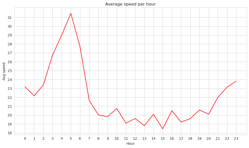
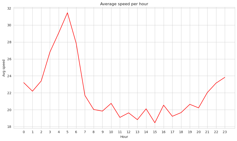
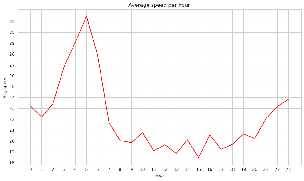
Study 1: Average speed of taxis in terms of the hour

In this study we are going to calculate the average speed of NY taxis each hour of the day to be able to analyze the traffic in the city. We have done this study with data-frames, RDD, SQL and also with Pandas. We have carried out the following steps:

1. Converte trip distance from miles to kilometers.

2. Calculate speed by dividing trip distance over trip duration calculated before.

3. We group by the hour of the day calculating the mean of the speed.

4. We plot the results.

With Spark data-frames

taxis_df_copy = taxis_df.alias('taxis_df_copy')
taxis_df_copy.show(2)

+--------+--------------------+---------------------+---------------+-------------+----------+------------------+------------+------------+------------+-----------+-----+-------+----------+------------+---------------------+------------+-------------------+
|VendorID|tpep_pickup_datetime|tpep_dropoff_datetime|passenger_count|trip_distance|RatecodeID|store_and_fwd_flag|PULocationID|DOLocationID|payment_type|fare_amount|extra|mta_tax|tip_amount|tolls_amount|improvement_surcharge|total_amount|trip_duration_hours|
+--------+--------------------+---------------------+---------------+-------------+----------+------------------+------------+------------+------------+-----------+-----+-------+----------+------------+---------------------+------------+-------------------+
|       1| 2017-01-09 11:13:28|  2017-01-09 11:25:45|              1|          3.3|         1|                 N|         263|         161|           1|       12.5|  0.0|    0.5|       2.0|         0.0|                  0.3|        15.3|              0.205|
|       1| 2017-01-09 11:32:27|  2017-01-09 11:36:01|              1|          0.9|         1|                 N|         186|         234|           1|        5.0|  0.0|    0.5|      1.45|         0.0|                  0.3|        7.25|              0.059|
+--------+--------------------+---------------------+---------------+-------------+----------+------------------+------------+------------+------------+-----------+-----+-------+----------+------------+---------------------+------------+-------------------+
only showing top 2 rows

taxis_df_copy = taxis_df_copy.withColumn("trip_distance_km", round(taxis_df_copy["trip_distance"]*1.609344, 3))
taxis_df_copy = taxis_df_copy.withColumn("trip_speed_km_h",  round(taxis_df_copy['trip_distance_km'] / taxis_df_copy['trip_duration_hours'], 3))
taxis_df_copy = taxis_df_copy.withColumn("hour_time", date_format(from_unixtime(unix_timestamp("tpep_pickup_datetime", "yyyy-MM-dd HH:mm:ss")), "HH"))
hours_speed_df = taxis_df_copy.groupBy("hour_time").mean('trip_speed_km_h')
hours_speed_df = hours_speed_df.withColumn("hour_time", hours_speed_df["hour_time"].cast(IntegerType())) # Convert the "hour_time" column to integer type
start_time = time.time()
hours_speed_df_pd = hours_speed_df.toPandas()
end_time = time.time()
task1_spark_df_time = end_time - start_time
print('Time of task 1 with Spark data-frames', task1_spark_df_time)

Time of task 1 with Spark data-frames 2.0894644260406494

plt.figure(figsize=(10, 6))
sns.lineplot(x="hour_time", y="avg(trip_speed_km_h)", data=hours_speed_df_pd, color='red')
plt.xlabel("Hour")
plt.ylabel("Avg speed")
plt.title("Average speed per hour")
plt.xticks(range(0,24), rotation=0) 
min = np.round(hours_speed_df_pd["avg(trip_speed_km_h)"].min())
max = np.round(hours_speed_df_pd["avg(trip_speed_km_h)"].max())
ysticks_ = np.unique(np.round(np.linspace(min, max, 15)))
plt.yticks(ysticks_) 
plt.tight_layout()
plt.show()

With Spark RDD

taxis_df_copy = taxis_df.alias('taxis_df_copy')
taxis_df_copy.show(2)

+--------+--------------------+---------------------+---------------+-------------+----------+------------------+------------+------------+------------+-----------+-----+-------+----------+------------+---------------------+------------+-------------------+
|VendorID|tpep_pickup_datetime|tpep_dropoff_datetime|passenger_count|trip_distance|RatecodeID|store_and_fwd_flag|PULocationID|DOLocationID|payment_type|fare_amount|extra|mta_tax|tip_amount|tolls_amount|improvement_surcharge|total_amount|trip_duration_hours|
+--------+--------------------+---------------------+---------------+-------------+----------+------------------+------------+------------+------------+-----------+-----+-------+----------+------------+---------------------+------------+-------------------+
|       1| 2017-01-09 11:13:28|  2017-01-09 11:25:45|              1|          3.3|         1|                 N|         263|         161|           1|       12.5|  0.0|    0.5|       2.0|         0.0|                  0.3|        15.3|              0.205|
|       1| 2017-01-09 11:32:27|  2017-01-09 11:36:01|              1|          0.9|         1|                 N|         186|         234|           1|        5.0|  0.0|    0.5|      1.45|         0.0|                  0.3|        7.25|              0.059|
+--------+--------------------+---------------------+---------------+-------------+----------+------------------+------------+------------+------------+-----------+-----+-------+----------+------------+---------------------+------------+-------------------+
only showing top 2 rows

def calculate_elapsed_hours(start_time, end_time):
    elapsed_time = (end_time - start_time).total_seconds() / 3600
    return np.round(elapsed_time,3)

trip_distance_rdd = taxis_df_copy.select('trip_distance').rdd.map(lambda x: x[0])
trip_distance_km_rdd = trip_distance_rdd.map(lambda x : np.round(x*1.609344, 3))
tpep_dropoff_datetime_rdd = taxis_df_copy.select('tpep_dropoff_datetime').rdd.map(lambda x: x[0])
tpep_pickup_datetime_rdd = taxis_df_copy.select('tpep_pickup_datetime').rdd.map(lambda x: x[0])
datetime_rdd = taxis_df_copy.select('tpep_pickup_datetime', 'tpep_dropoff_datetime').rdd.map(lambda x: (x[0],x[1]))
trip_duration_rdd = datetime_rdd.map(lambda x : calculate_elapsed_hours(x[0], x[1]))
trip_distance_time_rdd = trip_distance_km_rdd.zip(trip_duration_rdd)
trip_speed_rdd = trip_distance_time_rdd.map(lambda x : np.round(x[0] / x[1], 3))
trip_hour_rdd = tpep_pickup_datetime_rdd.map(lambda x : x.hour)
key_hour_rdd = trip_hour_rdd.map(lambda x : (x,1))
trip_hour_sum_hour_rdd = key_hour_rdd.reduceByKey(lambda x,y : x + y)
trip_hour_speed_rdd = trip_hour_rdd.zip(trip_speed_rdd)
trip_hour_sum_speed_rdd = trip_hour_speed_rdd.reduceByKey(lambda x,y : np.round(x + y, 3)) 
avg_speed_hour_rdd = trip_hour_sum_hour_rdd.zip(trip_hour_sum_speed_rdd).map(lambda x : (np.round(x[1][1] / x[0][1], 3))) 
hours_new_order_rdd = trip_hour_sum_hour_rdd.map(lambda x : x[0])
start_time = time.time()
avg_speed_hour_list = avg_speed_hour_rdd.collect()
hours_new_order_list = hours_new_order_rdd.collect()
end_time = time.time()
task1_spark_rdd_time = end_time - start_time
print('Time of task 1 with Spark RDDs', task1_spark_rdd_time)

Time of task 1 with Spark RDDs 15.936208009719849

plt.figure(figsize=(10, 6))
sns.lineplot(x=hours_new_order_list, y=avg_speed_hour_list, color='red')
plt.xlabel("Hour")
plt.ylabel("Avg speed")
plt.title("Average speed per hour")
plt.xticks(range(0,24), rotation=0) 
#min = np.round(hours_speed_df_pd["avg(trip_speed_km_h)"].min())
#max = np.round(hours_speed_df_pd["avg(trip_speed_km_h)"].max())
#ysticks_ = np.unique(np.round(np.linspace(min, max, 15)))
#plt.yticks(ysticks_) 
plt.tight_layout()
plt.show()

With Spark SQL

taxis_df_copy = taxis_df.alias('taxis_df_copy')
taxis_df_copy.show(2)

+--------+--------------------+---------------------+---------------+-------------+----------+------------------+------------+------------+------------+-----------+-----+-------+----------+------------+---------------------+------------+-------------------+
|VendorID|tpep_pickup_datetime|tpep_dropoff_datetime|passenger_count|trip_distance|RatecodeID|store_and_fwd_flag|PULocationID|DOLocationID|payment_type|fare_amount|extra|mta_tax|tip_amount|tolls_amount|improvement_surcharge|total_amount|trip_duration_hours|
+--------+--------------------+---------------------+---------------+-------------+----------+------------------+------------+------------+------------+-----------+-----+-------+----------+------------+---------------------+------------+-------------------+
|       1| 2017-01-09 11:13:28|  2017-01-09 11:25:45|              1|          3.3|         1|                 N|         263|         161|           1|       12.5|  0.0|    0.5|       2.0|         0.0|                  0.3|        15.3|              0.205|
|       1| 2017-01-09 11:32:27|  2017-01-09 11:36:01|              1|          0.9|         1|                 N|         186|         234|           1|        5.0|  0.0|    0.5|      1.45|         0.0|                  0.3|        7.25|              0.059|
+--------+--------------------+---------------------+---------------+-------------+----------+------------------+------------+------------+------------+-----------+-----+-------+----------+------------+---------------------+------------+-------------------+
only showing top 2 rows

taxis_df_copy.createOrReplaceTempView('taxis_df_copy') 
taxis_df_copy = spark.sql("SELECT *, round(trip_distance*1.609344, 3) as trip_distance_km FROM taxis_df_copy")
taxis_df_copy.createOrReplaceTempView('taxis_df_copy') 
taxis_df_copy = spark.sql("SELECT *, round(trip_distance_km / trip_duration_hours, 3) as trip_speed_km_h FROM taxis_df_copy") 
taxis_df_copy.createOrReplaceTempView('taxis_df_copy') 
taxis_df_copy = spark.sql("SELECT *, hour(tpep_pickup_datetime) as hour_time FROM taxis_df_copy")
taxis_df_copy.createOrReplaceTempView('taxis_df_copy') 
hours_speed_df = spark.sql("SELECT CAST(hour_time AS INT) AS hour_time, avg(trip_speed_km_h) FROM taxis_df_copy GROUP BY hour_time") 
start_time = time.time()
hours_speed_df_pd = hours_speed_df.toPandas()
end_time = time.time()
task1_spark_sql_time = end_time - start_time
print('Time of task 1 with Spark SQL', task1_spark_sql_time)

Time of task 1 with Spark SQL 2.2889022827148438

plt.figure(figsize=(10, 6))
sns.lineplot(x="hour_time", y="avg(trip_speed_km_h)", data=hours_speed_df_pd, color='red')
plt.xlabel("Hour")
plt.ylabel("Avg speed")
plt.title("Average speed per hour")
plt.xticks(range(0,24), rotation=0) 
min = np.round(hours_speed_df_pd["avg(trip_speed_km_h)"].min())
max = np.round(hours_speed_df_pd["avg(trip_speed_km_h)"].max())
ysticks_ = np.unique(np.round(np.linspace(min, max, 15)))
plt.yticks(ysticks_) 
plt.tight_layout()
plt.show()

With Pandas

taxis_df_pd = pd.read_csv(r"./Data/taxis.csv")
taxis_df_pd.head()

	VendorID	tpep_pickup_datetime	tpep_dropoff_datetime	passenger_count	trip_distance	RatecodeID	store_and_fwd_flag	PULocationID	DOLocationID	payment_type	fare_amount	extra	mta_tax	tip_amount	tolls_amount	improvement_surcharge	total_amount
0	1	2017-01-09 11:13:28	2017-01-09 11:25:45	1	3.30	1	N	263	161	1	12.5	0.0	0.5	2.00	0.0	0.3	15.30
1	1	2017-01-09 11:32:27	2017-01-09 11:36:01	1	0.90	1	N	186	234	1	5.0	0.0	0.5	1.45	0.0	0.3	7.25
2	1	2017-01-09 11:38:20	2017-01-09 11:42:05	1	1.10	1	N	164	161	1	5.5	0.0	0.5	1.00	0.0	0.3	7.30
3	1	2017-01-09 11:52:13	2017-01-09 11:57:36	1	1.10	1	N	236	75	1	6.0	0.0	0.5	1.70	0.0	0.3	8.50
4	2	2017-01-01 00:00:00	2017-01-01 00:00:00	1	0.02	2	N	249	234	2	52.0	0.0	0.5	0.00	0.0	0.3	52.80

taxis_df_pd.shape

(971010, 17)

Data cleaning with Pandas

start_time = time.time()

• Removing trips (rows) with zero (0) duration:

taxis_df_pd['tpep_pickup_datetime'] = pd.to_datetime(taxis_df_pd['tpep_pickup_datetime'])
taxis_df_pd['tpep_dropoff_datetime'] = pd.to_datetime(taxis_df_pd['tpep_dropoff_datetime'])
taxis_df_pd['trip_duration_hours'] = ((taxis_df_pd['tpep_dropoff_datetime'] - taxis_df_pd['tpep_pickup_datetime']).dt.total_seconds() / 3600).round(3)
taxis_df_pd = taxis_df_pd.loc[taxis_df_pd['trip_duration_hours'] > 0, :]

• Removing rows with total_amount, tip_amount, mta_tax, fare_amount <= 0.

for col in ['total_amount', 'fare_amount'] :

    taxis_df_pd = taxis_df_pd.loc[taxis_df_pd[col] > 0, :]

for col in ['tip_amount', 'mta_tax'] :

    taxis_df_pd = taxis_df_pd.loc[taxis_df_pd[col] >= 0, :]

• Removing upper outliers in total_amount, tolls_amount.

for col in ['total_amount', 'tolls_amount'] :

    Q75 = taxis_df_pd[col].quantile(0.75) 
    Q25 = taxis_df_pd[col].quantile(0.25) 
    IQR = Q75 - Q25
    upper_bound = Q75 + 2.5*IQR
    taxis_df_pd = taxis_df_pd.loc[taxis_df_pd[col] <= upper_bound, :]

end_time = time.time()
data_cleaning_pandas_time = end_time - start_time
print('Data cleaning with pandas: ', data_cleaning_pandas_time)

Data cleaning with pandas:  0.8886573314666748

taxis_df_pd.shape

(900387, 18)

Performing the task

start_time = time.time()
taxis_df_pd['trip_distance_km'] = (taxis_df_pd["trip_distance"]*1.609344).round(3)
taxis_df_pd['trip_speed_km_h'] = (taxis_df_pd["trip_distance_km"] / taxis_df_pd['trip_duration_hours']).round(3)
taxis_df_pd['hour_time'] =  taxis_df_pd['tpep_pickup_datetime'].dt.hour
hours_speed_df_pd = taxis_df_pd.groupby(by='hour_time')['trip_speed_km_h'].mean()
end_time = time.time()
task1_pandas_time = end_time - start_time
print('Time of task 1 with pandas: ', task1_pandas_time)

Time of task 1 with pandas:  0.0503997802734375

plt.figure(figsize=(10, 6))
sns.lineplot(x=hours_speed_df_pd.index, y=hours_speed_df_pd.values, color='red')
plt.xlabel("Hour")
plt.ylabel("Avg speed")
plt.title("Average speed per hour")
plt.xticks(range(0,24), rotation=0) 
min = np.round(hours_speed_df_pd.values.min())
max = np.round(hours_speed_df_pd.values.max())
ysticks_ = np.unique(np.round(np.linspace(min, max, 15)))
plt.yticks(ysticks_) 
plt.tight_layout()
plt.show()

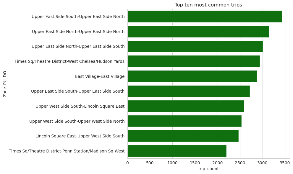
Study 2: Most common taxi trips

In this study we have analyzed the most common taxi trips. We have used Spark Data Frame.
We have followed the nesxt steps:

1. Read the file “zones.csv” that provides the borough and zone of the pickup and dropoff codes.

2. Filter the unknown trips in the zones dataset.

3. Group by pickup and dropoff location ids counting the records and ordering by this count.

4. Join both datasets, trips and zones, in order to get the borough and zones of the pickup and dropoff location ids.

5. Order by trip count the final result to get the most common trips.

6. Show the 10 most common trips.

7. Plot the results.

zones_df = spark.read.format("csv").option("inferSchema", "true").option("timestampFormat","yyyy-MM-dd HH:mm:ss").option("header", "true").option("mode", "DROPMALFORMED").load(r"./Data/zones.csv")
zones_df = zones_df.filter(zones_df['LocationID'] < 264)
group_by_df = taxis_df.groupBy('PULocationID', 'DOLocationID').agg(count('*').alias('trip_count')).orderBy('trip_count', ascending=False)
PU_joined_df = group_by_df.join(zones_df, group_by_df['PULocationID'] == zones_df['LocationID'], 'inner')\
    .select('PULocationID', 'DOLocationID', 'LocationID', 'trip_count', 'Borough', 'Zone')\
    .withColumnRenamed('Borough', 'Borough_PU')\
    .withColumnRenamed('Zone', 'Zone_PU')\
    .withColumnRenamed('trip_count', 'trip_count_PU')
DO_joined_df = group_by_df.join(zones_df, group_by_df['DOLocationID'] == zones_df['LocationID'], 'inner').select('PULocationID', 'DOLocationID', 'LocationID', 'trip_count', 'Borough', 'Zone').withColumnRenamed('Borough', 'Borough_DO').withColumnRenamed('Zone', 'Zone_DO')
zones_trips_df = PU_joined_df.join(DO_joined_df, (PU_joined_df['PULocationID'] == DO_joined_df['PULocationID']) & (PU_joined_df['DOLocationID'] == DO_joined_df['DOLocationID']), 'inner').select('Borough_PU', 'Zone_PU', 'Borough_DO', 'Zone_DO', 'trip_count')
zones_trips_sorted_df = zones_trips_df.orderBy('trip_count', ascending=False)
start_time = time.time()
zones_trips_sorted_df.show(10)
end_time = time.time()
task2_spark_df_time = end_time - start_time

+----------+--------------------+----------+--------------------+----------+
|Borough_PU|             Zone_PU|Borough_DO|             Zone_DO|trip_count|
+----------+--------------------+----------+--------------------+----------+
| Manhattan|Upper East Side S...| Manhattan|Upper East Side N...|      3433|
| Manhattan|Upper East Side N...| Manhattan|Upper East Side N...|      3149|
| Manhattan|Upper East Side N...| Manhattan|Upper East Side S...|      3005|
| Manhattan|Times Sq/Theatre ...| Manhattan|West Chelsea/Huds...|      2940|
| Manhattan|        East Village| Manhattan|        East Village|      2877|
| Manhattan|Upper East Side S...| Manhattan|Upper East Side S...|      2719|
| Manhattan|Upper West Side S...| Manhattan| Lincoln Square East|      2594|
| Manhattan|Upper West Side S...| Manhattan|Upper West Side N...|      2536|
| Manhattan| Lincoln Square East| Manhattan|Upper West Side S...|      2470|
| Manhattan|Times Sq/Theatre ...| Manhattan|Penn Station/Madi...|      2202|
+----------+--------------------+----------+--------------------+----------+
only showing top 10 rows

print('Time task 2 with Spark data-frames: ', task2_spark_df_time)

Time task 2 with Spark data-frames:  5.124625205993652

from pyspark.sql.functions import col
zones_trips_sorted_df = zones_trips_sorted_df.withColumn('Zone_PU_DO', concat(col('Zone_PU'), lit('-'), col('Zone_DO')))
zones_trips_sorted_df_pd = zones_trips_sorted_df.toPandas()

plt.figure(figsize=(10, 6))
sns.barplot(y="Zone_PU_DO", x="trip_count", data=zones_trips_sorted_df_pd.head(10), color='green')
plt.xlabel("trip_count")
plt.ylabel("Zone_PU_DO")
plt.title("Top ten most common trips")
plt.xticks(rotation=0) 
# min = np.round(hours_speed_df_pd["avg(trip_speed_km_h)"].min())
# max = np.round(hours_speed_df_pd["avg(trip_speed_km_h)"].max())
# ysticks_ = np.unique(np.round(np.linspace(min, max, 15)))
# plt.yticks(ysticks_) 
plt.tight_layout()
plt.show()

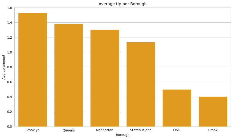
Study 3: Average of tips per borough

In this study we have analyzed the average of tips per pickup borough. We have used Spark SQL.
We have followed the nesxt steps:

1. Read the file “zones.csv” that provides the borough and zone of the pickup and dropoff codes.

2. Join both datasets, trips and zones, in order to get the borough and average trip amount excluding the unknown zones, grouping by borough and ordering by the average trip amount .

3. Show the results.

4. Plot the results.

zones_df = spark.read.format("csv").option("inferSchema", "true").option("timestampFormat","yyyy-MM-dd HH:mm:ss").option("header", "true").option("mode", "DROPMALFORMED").load(r"./Data/zones.csv")

zones_df.createOrReplaceTempView('zones_df') 
taxis_df.createOrReplaceTempView('taxis_df') 
join_df = spark.sql("SELECT Borough, AVG(tip_amount) AS tip_amount_avg FROM taxis_df JOIN zones_df ON PULocationID = LocationID WHERE PULocationID < 264  GROUP BY Borough ORDER BY AVG(tip_amount) DESC")
start_time = time.time()
join_df.show(10)
end_time = time.time()
task3_spark_sql_time = end_time - start_time

+-------------+------------------+
|      Borough|    tip_amount_avg|
+-------------+------------------+
|     Brooklyn|1.5295506094329612|
|       Queens|1.3814509977827034|
|    Manhattan|1.3054620174908678|
|Staten Island|1.1371428571428572|
|          EWR|               0.5|
|        Bronx|0.4036954915003696|
+-------------+------------------+

print('Time of task 3 with Spark SQL', task3_spark_sql_time)

Time of task 3 with Spark SQL 2.7581818103790283

join_df_pd = join_df.toPandas()

plt.figure(figsize=(10, 6))
sns.barplot(x="Borough", y="tip_amount_avg", data=join_df_pd, color='orange')
plt.xlabel("Borough")
plt.ylabel("Avg tip amount")
plt.title("Average tip per Borough")
# plt.xticks(range(0,24), rotation=0) 
# min = np.round(hours_speed_df_pd["avg(trip_speed_km_h)"].min())
# max = np.round(hours_speed_df_pd["avg(trip_speed_km_h)"].max())
# ysticks_ = np.unique(np.round(np.linspace(min, max, 15)))
# plt.yticks(ysticks_) 
plt.tight_layout()
plt.show()

Time Analysis

Spark and number of cores

In this section we have analyzed both the different times of execution and speed-up of the different processes.

• We have done differentes measurements using distinct number of cores: 1, 2, 4, 6, 8 and 10 (all).

• We have created a table with all this measurements in order to analyze them and make different plots to show the results.

cores = np.array([1,2,4,6,8,10])
data_cleaning_spark_df_time = np.array([17.51055, 11.5567, 7.8198, 7.1175,  7.0512 , 6.4139])
task1_spark_df_time = np.array([5.902377, 3.45250, 2.49201, 2.60570,  2.2375 , 1.8649])
task1_spark_rdd_time = np.array([34.256966 , 21.998392 , 18.01433 , 17.94407 ,  16.6878   , 16.96136 ])
task1_spark_sql_time = np.array([6.7926690, 3.687486, 2.9901852, 2.642264,  2.2889 , 2.14359])
task2_spark_df_time = np.array([11.040179, 6.647932, 5.729816, 5.35511, 5.1246 , 5.066134])
task3_spark_sql_time = np.array([6.1619, 3.180148, 2.62037, 2.56909, 2.4121, 2.15730])

df_times = dict()
df_times['cores'] = cores
df_times['data_cleaning_spark_df_time'] = data_cleaning_spark_df_time
df_times['task1_spark_df_time'] = task1_spark_df_time
df_times['task1_spark_rdd_time'] = task1_spark_rdd_time
df_times['task1_spark_sql_time'] = task1_spark_sql_time
df_times['task2_spark_df_time'] = task2_spark_df_time
df_times['task3_spark_sql_time'] = task3_spark_sql_time
df_times = pd.DataFrame(df_times)

df_times

	cores	data_cleaning_spark_df_time	task1_spark_df_time	task1_spark_rdd_time	task1_spark_sql_time	task2_spark_df_time	task3_spark_sql_time
0	1	17.51055	5.902377	34.256966	6.792669	11.040179	6.161900
1	2	11.55670	3.452500	21.998392	3.687486	6.647932	3.180148
2	4	7.81980	2.492010	18.014330	2.990185	5.729816	2.620370
3	6	7.11750	2.605700	17.944070	2.642264	5.355110	2.569090
4	8	7.05120	2.237500	16.687800	2.288900	5.124600	2.412100
5	10	6.41390	1.864900	16.961360	2.143590	5.066134	2.157300

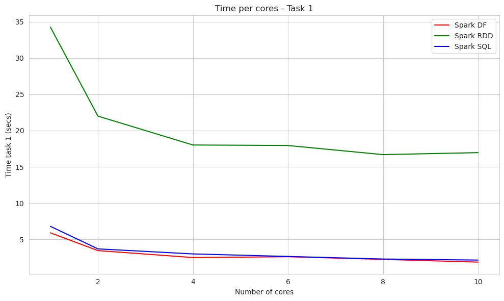
The following plot compares the time per cores of the first study with df, RDD or SQL.

plt.figure(figsize=(10, 6))
sns.lineplot(x='cores', y='task1_spark_df_time', data=df_times, color='red', label='Spark DF')
sns.lineplot(x='cores', y='task1_spark_rdd_time', data=df_times, color='green', label='Spark RDD')
sns.lineplot(x='cores', y='task1_spark_sql_time', data=df_times, color='blue', label='Spark SQL')
plt.xlabel("Number of cores")
plt.ylabel("Time task 1 (secs)")
plt.title("Time per cores - Study 1")
plt.xticks(rotation=0) 
plt.tight_layout()
plt.legend()
plt.show()

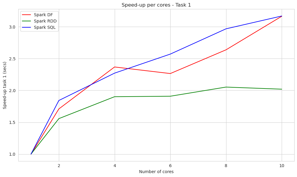
We calculate the speed up of all the processes by dividing the time of execution of one core by the time of execution with the cores used.

df_speed_up = pd.DataFrame(index=range(len(df_times)))

for col_name in df_times.columns:

    if col_name == 'cores':

        df_speed_up[col_name] = df_times[col_name]

    else:

        base_time = df_times.loc[df_times['cores'] == 1, col_name].iloc[0]
        df_speed_up[col_name] = base_time / df_times[col_name] 

df_speed_up

	cores	data_cleaning_spark_df_time	task1_spark_df_time	task1_spark_rdd_time	task1_spark_sql_time	task2_spark_df_time	task3_spark_sql_time
0	1	1.000000	1.000000	1.000000	1.000000	1.000000	1.000000
1	2	1.515186	1.709595	1.557249	1.842087	1.660694	1.937614
2	4	2.239258	2.368521	1.901651	2.271655	1.926795	2.351538
3	6	2.460211	2.265179	1.909097	2.570776	2.061616	2.398476
4	8	2.483343	2.637934	2.052815	2.967657	2.154349	2.554579
5	10	2.730094	3.164983	2.019706	3.168828	2.179212	2.856302

This plot compares the speed up per cores of the first study with Spark DF, RDD and SQL.

plt.figure(figsize=(10, 6))
sns.lineplot(x='cores', y='task1_spark_df_time', data=df_speed_up, color='red', label='Spark DF')
sns.lineplot(x='cores', y='task1_spark_rdd_time', data=df_speed_up, color='green', label='Spark RDD')
sns.lineplot(x='cores', y='task1_spark_sql_time', data=df_speed_up, color='blue', label='Spark SQL')
plt.xlabel("Number of cores")
plt.ylabel("Speed-up task 1 (secs)")
plt.title("Speed-up per cores - Study 1")
plt.xticks(rotation=0) 
plt.tight_layout()
plt.legend()
plt.show()

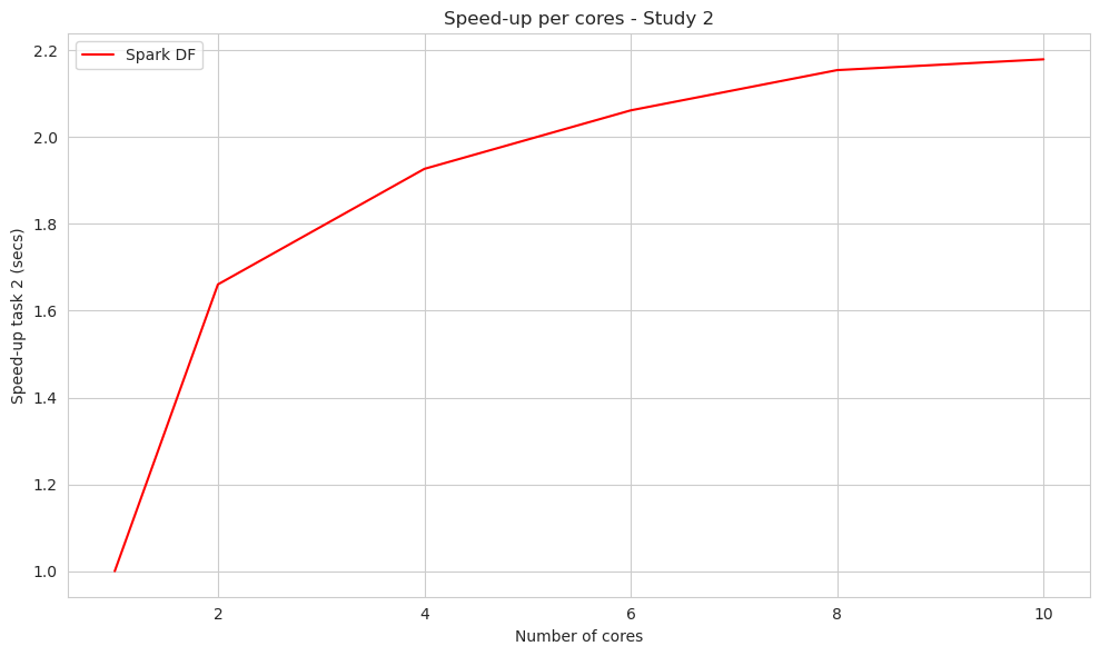
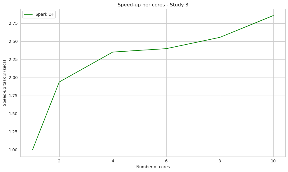
The plots below show the speedup of the other studies and the clean up process per cores.

plt.figure(figsize=(10, 6))
sns.lineplot(x='cores', y='task2_spark_df_time', data=df_speed_up, color='red', label='Spark DF')
plt.xlabel("Number of cores")
plt.ylabel("Speed-up task 2 (secs)")
plt.title("Speed-up per cores - Study 2")
plt.xticks(rotation=0) 
plt.tight_layout()
plt.legend()
plt.show()

plt.figure(figsize=(10, 6))
sns.lineplot(x='cores', y='task3_spark_sql_time', data=df_speed_up, color='green', label='Spark DF')
plt.xlabel("Number of cores")
plt.ylabel("Speed-up task 3 (secs)")
plt.title("Speed-up per cores - Study 3")
plt.xticks(rotation=0) 
plt.tight_layout()
plt.legend()
plt.show()

Conclusions

In the first study, we compared three different methods and represented their efficiency in the same plot, focusing on time and speed-up. The time plot allowed us to assess the efficiency of these methods, and it was evident that RDDs performed the slowest, while the other methods showed similar performance, especially with a higher number of cores. Surprisingly, we did not observe the expected improvements in Spark RDDs, indicating that the dataset size might not be sufficient. In the next section, we plan to explore this further with a different dataset to better understand this behavior.

The speed-up analysis in the subsequent plot revealed more promising results with a higher number of cores, which is an expected outcome. However, once again, RDDs exhibited a slower increase in speed-up as the number of cores increased.

In our subsequent studies, we focused solely on the speed-up analysis because it provides valuable information. In both of these studies, we observed an increase in speed-up as the number of cores used increased. Although each method displayed a slightly different slope in its evolution, both methods demonstrated good scalability with the increasing number of cores.

Spark vs Pandas vs Polars

The next plot has been build with information extracted after a meticulous procedure that we are going to expose now:

• We have consider the provided data-set as baseline (which has 1 million rows, approx), then, we have build bigger version of it, just making copies and concatenating them. Following this technique we have created other four data-set, with the same columns of the original, but with much more rows, specifically, 15, 62, 124 and 186 millions, respectively.

• After that, we have perform data reading, cleaning and study 1 with Spark-DF, Spark-SQL, Spark-RDD, Pandas and Polars, with each one of those five data-sets, measuring execution time carefully, and, then, we have repeat the process three times, in order to compute an average metric. As extra detail, Spark-RDD has only been used with 1M and 15M data-sets, due to the extremely high computational cost that we have experimented with this approach.

• Once the previous step is carried out, we have an average execution time for each combination of task (data reading, cleaning and study 1), approach (Spark-DF, Spark-SQL, Spark-RDD, Pandas and Polars) and data-set (1M, 15M, 62M, 124M, 186M).

• Finally, we have used the last information in a smart way for building up the next plot, which summarize in a clever and beautiful way the results obtained with our comparative analysis.

import pickle
from itertools import product

# Open a dictionary saved as a pickle
with open('Spark_times_df_dict.pickle', 'rb') as file:
    # Read back the pickled file
    Spark_times_df_dict = pickle.load(file)

# Open a dictionary saved as a pickle
with open('Pandas_times_df_dict.pickle', 'rb') as file:
    # Read back the pickled file
    Pandas_times_df_dict = pickle.load(file)

# Open a dictionary saved as a pickle
with open('Polars_times_df_dict.pickle', 'rb') as file:
    # Read back the pickled file
    Polars_times_df_dict = pickle.load(file)

for data in ['taxis.csv', 'taxis_15M.csv', 'taxis_62M.csv', 'taxis_124M.csv', 'taxis_186M.csv'] :

    if data in ['taxis.csv', 'taxis_15M.csv'] :
        Spark_times_df_dict[data].columns = ['data_reading_Spark-DF_time', 'data_cleaning_Spark-DF_time', 'task1_Spark-DF_time', 'task1_Spark-RDD_time', 'task1_Spark-SQL_time'] 
    else :
        Spark_times_df_dict[data].columns = ['data_reading_Spark-DF_time', 'data_cleaning_Spark-DF_time', 'task1_Spark-DF_time', 'task1_Spark-SQL_time'] 
          
    Pandas_times_df_dict[data].columns = ['data_reading_Pandas_time', 'data_cleaning_Pandas_time', 'task1_Pandas_time'] 
    Polars_times_df_dict[data].columns = ['data_reading_Polars_time', 'data_cleaning_Polars_time', 'task1_Polars_time'] 

data_names = ['taxis.csv', 'taxis_15M.csv', 'taxis_62M.csv', 'taxis_124M.csv', 'taxis_186M.csv']
methods = ['Spark-DF', 'Pandas', 'Polars', 'Spark-RDD', 'Spark-SQL']
tasks = ['data_reading', 'data_cleaning', 'task1']
def df_name(x) :
    if x in ['Spark-DF', 'Spark-RDD', 'Spark-SQL'] :
        return x[0:5]
    else :
        return x      

avg_time= dict()
for task in tasks :
    avg_time[task] = dict()

for task in tasks :
    if task in ['data_reading', 'data_cleaning']:
        for method in ['Spark-DF', 'Pandas', 'Polars'] :
            avg_time[task][method] = dict()
    else:
        for method in methods:
            avg_time[task][method] = dict()

times_df_dict = dict()
for name in ['Spark', 'Pandas', 'Polars'] :
    times_df_dict[name] = globals()[f'{name}_times_df_dict']

#########################################################################################

filtered_product = [(method, data, task) for method, data, task in product(methods, data_names, tasks) 
                    if not (method == 'Spark-RDD' and task in ['data_reading', 'data_cleaning'])
                    and not (method == 'Spark-SQL' and task in ['data_reading', 'data_cleaning'])]

for method, data, task in filtered_product :

    if method == 'Spark-RDD' and data in ['taxis_62M.csv', 'taxis_124M.csv', 'taxis_186M.csv']: 

        avg_time[task][method][data] = np.NaN

    else :
        
        avg_time[task][method][data] = times_df_dict[df_name(method)][data].describe().loc['mean', f'{task}_{method}_time']

#########################################################################################

def total_time_v1(method, data) :
    return np.sum([avg_time[task][method][data] for task in tasks])

def total_time_v2(method) :
    return {data : total_time_v1(method, data=data) for data in data_names}

avg_time['all_tasks'] = dict()

for method in ['Spark-DF', 'Pandas', 'Polars'] :

    avg_time['all_tasks'][method] = total_time_v2(method)

# Define the number of rows and columns for the matrix plot
num_cols = 4  # You can adjust the number of columns as needed
n_tasks = len(avg_time)
num_rows = int(np.ceil(n_tasks / num_cols))

data_size = ['1M', '15M', '62M', '124M', '186M']
titles = ['Data reading', 'Data cleaning', 'Study 1', 'All the tasks']

# Create a subplot with the specified number of rows and columns
fig, axes = plt.subplots(num_rows, num_cols, figsize=(21, 6))

# Flatten the axes array to make it easier to iterate
axes = axes.flatten()

n_methods = 5 # (spark-df, spark-sql, spark-rdd pandas, polars)
colors = sns.color_palette("tab10", n_methods)

# Loop through each 'geo' and create a subplot in the matrix
for (i, task), title in zip(enumerate(avg_time.keys()), titles) :

    ax = axes[i]  # Get the current axis
    for method, color in zip(avg_time[task].keys(), colors) :
        sns.lineplot(x=data_size, y=avg_time[task][method].values(), color=color, marker='o', markersize=6, linestyle='-', linewidth=2, label=method, ax=ax)    
    ax.set_xlabel("Data size (millions)", fontsize=12)
    ax.set_ylabel("Average time (seconds)", fontsize=12)
    ax.tick_params(axis='x', rotation=0)
    ax.tick_params(axis='y', rotation=0)
    ax.set_title(title, fontsize=14, weight='normal', style='italic', color='black')
    ax.get_legend().remove()  # Remove individual subplot legends
    if i == 2 : # Getting the labels of the third plot (the one with more labels), for build a general legend.
        handles, labels = ax.get_legend_handles_labels() 

# Remove any unused subplots in case the number of 'geo' values is less than num_rows * num_cols
for j in range(len(avg_time), num_rows * num_cols):
    fig.delaxes(axes[j])

# Add a shared legend outside of the subplots
fig.legend(handles, methods, loc='lower center', bbox_to_anchor=(0.5, -0.1), ncol=n_methods, fontsize=13)

plt.suptitle('Spark vs Pandas vs Polars - Time comparison', fontsize=16, y=0.99, weight='bold', style='italic', color='black', alpha=0.9) # Establishing a general tittle for the plot.
plt.subplots_adjust(hspace=1, wspace=0.3) # Adjust vertical (hspace) and horizontal (wspace) spacing
# fig.savefig('Spark_Pandas_Polars' + '.jpg', format='jpg', dpi=600, bbox_inches="tight")
# plt.tight_layout()
plt.show()

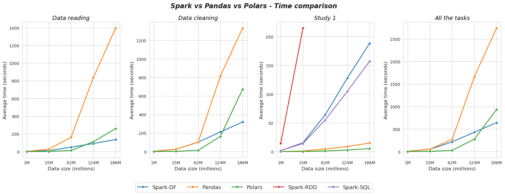
Some conclusions from the plot:

• Pandas is similar than Spark in terms of computation time when the dataset size is moderate (1M, 15M), but there is a size at which Spark starts to be more efficient than Pandas (62M, 124M, 186M) or, rather, Pandas becomes too slow a library.

• Polars have a similar behavior than Pandas for moderate data sets (1M, 15M), but for real big data sets (62M, 124M, 186M) the performance of Polars in terms of time is much better that the Pandas one. On the other hand, Polars is also better than Spark in almost all the cases, even when we have quite big data (124M), but when the amount of data is massive (186M), the great power of Spark appears on the scene, achieving better results than Polars.

• The power of Spark parallelization is shown when the data is large enough (64M, 124M, 186M), and this analysis suggests that, the more data we have, the better results Spark will achieve in terms of time, compared to Pandas and Polars.